This repository contains code and trained models for the paper Certified Adversarial Robustness via Randomized Smoothing by Jeremy Cohen, Elan Rosenfeld, and Zico Kolter.
Randomized smoothing is a provable adversarial defense in L2 norm which scales to ImageNet. It's also SOTA on the smaller datasets like CIFAR-10 and SVHN where other provable L2-robust classifiers are viable.
First, you train a neural network f with Gaussian data augmentation at variance σ2. Then you leverage f to create a new, "smoothed" classifier g, defined as follows: g(x) returns the class which f is most likely to return when x is corrupted by isotropic Gaussian noise with variance σ2.
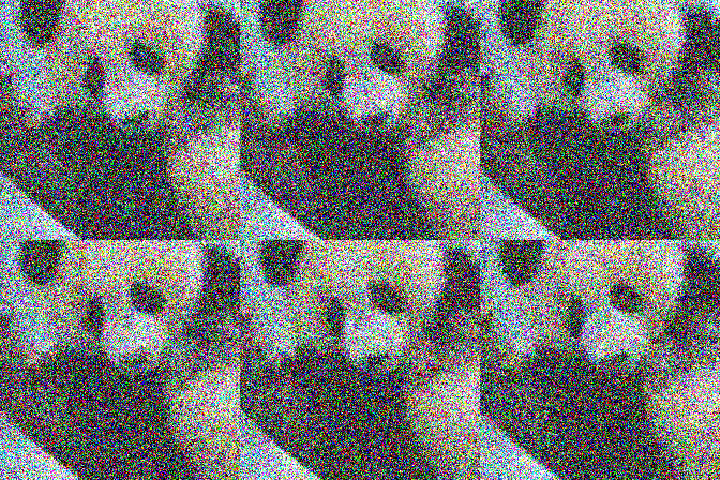
For example, let x be the image above on the left. Suppose that when f classifies x corrupted by Gaussian noise (the GIF on the right), f returns "panda" 98% of the time and "gibbon" 2% of the time. Then the prediction of g at x is defined to be "panda."
Interestingly, g is provably robust within an L2 norm ball around x, in the sense that for any perturbation δ with sufficiently small L2 norm, g(x+δ) is guaranteed to be "panda." In this particular example, g will be robust around x within an L2 radius of σ Φ-1(0.98) ≈ 2.05 σ, where Φ-1 is the inverse CDF of the standard normal distribution.
In general, suppose that when f classifies noisy corruptions of x, the class "panda" is returned with probability p (with p > 0.5). Then g is guaranteed to classify "panda" within an L2 ball around x of radius σ Φ-1(p).
We know that f classifies noisy corruptions of x as "panda" with probability 0.98. An equivalent way of phrasing this that the Gaussian distribution N(x, σ2I) puts measure 0.98 on the decision region of class "panda," defined as the set {x': f(x') = "panda"}. You can prove that no matter how the decision regions of f are "shaped", for any δ with ||δ||2 < σ Φ-1(0.98), the translated Gaussian N(x+δ, σ2I) is guaranteed to put measure > 0.5 on the decision region of class "panda," implying that g(x+δ) = "panda."
There's one catch: it's not possible to actually evaluate the smoothed classifer g. This is because it's not possible to exactly compute the probability distribution over the classes when f's input is corrupted by Gaussian noise. For the same reason, it's not possible to exactly compute the radius in which g is provably robust.
Instead, we give Monte Carlo algorithms for both
- prediction: evaluating g(x)
- certification: computing the L2 radius in which g is robust around x
which are guaranteed to return a correct answer with arbitrarily high probability.
The prediction algorithm does this by abstaining from making any prediction when it's a "close call," e.g. if 510 noisy corruptions of x were classified as "panda" and 490 were classified as "gibbon." Prediction is pretty cheap, since you don't need to use very many samples. For example, with our ImageNet classifier, making a prediction using 1000 samples took 1.5 seconds, and our classifier abstained 3% of the time.
On the other hand, certification is pretty slow, since you need a lot of samples to say with high probability that the measure under N(x, σ2I) of the "panda" decision region is close to 1. In our experiments we used 100,000 samples, so making each certification took 150 seconds.
Randomized smoothing was first proposed in Certified Robustness to Adversarial Examples with Differential Privacy and later improved upon in Second-Order Adversarial Attack and Certified Robustness. We simply tightened the analysis and showed that it outperforms the other provably L2-robust classifiers that have been proposed in the literature.
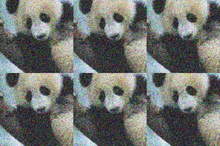
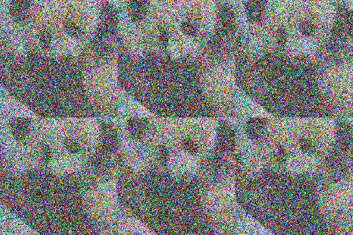
We constructed three randomized smoothing classifiers for ImageNet, with the hyperparameter σ set to 0.25, 0.50, and 1.00. Here's what the panda image looks like under these three noise levels:
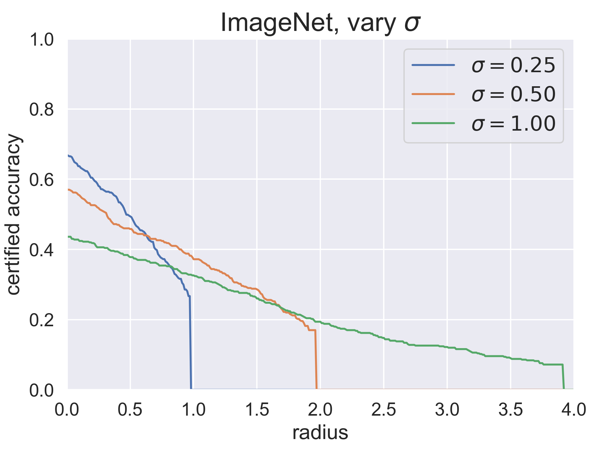
The plot below shows the certified top-1 accuracy at various radii of these three classifiers. The "certified accuracy" of a classifier g at radius r is defined as test set accuracy that g will provably attain under any possible adversarial attack with L2 norm less than r. As you can see, the hyperparameter σ controls a robustness/accuracy tradeoff: when σ is high, the standard accuracy is lower, but the classifier's correct predictions are robust within larger radii.
To put these numbers in context: on ImageNet, random guessing would achieve a top-1 accuracy of 0.001. A perturbation with L2 norm of 1.0 could change one pixel by 255, ten pixels by 80, 100 pixels by 25, or 1000 pixels by 8.
Here's the same data in tabular form. The best σ for each radius is denoted with an asterisk.
| r = 0.0 | r = 0.5 | r = 1.0 | r = 1.5 | r = 2.0 | r = 2.5 | r = 3.0 | |
|---|---|---|---|---|---|---|---|
| σ = 0.25 | 0.67* | 0.49* | 0.00 | 0.00 | 0.00 | 0.00 | 0.00 |
| σ = 0.50 | 0.57 | 0.46 | 0.38* | 0.28* | 0.00 | 0.00 | 0.00 |
| σ = 1.00 | 0.44 | 0.38 | 0.33 | 0.26 | 0.19* | 0.15* | 0.12* |
The contents of this repository are as follows:
- code/ contains the code for our experiments.
- data/ contains the raw data from our experiments.
- analysis/ contains the plots and tables, based on the contents of data, that are shown in our paper.
If you'd like to run our code, you need to download our models from here
and then move the directory models into the root directory of this repo.
Randomized smoothing is implemented in the Smooth class in core.py.
- To instantiate a smoothed clasifier g, use the constructor:
def __init__(self, base_classifier: torch.nn.Module, num_classes: int, sigma: float):
where base_classifier is a PyTorch module that implements f, num_classes is the number of classes in the output
space, and sigma is the noise hyperparameter σ
- To make a prediction at an input
x, call:
def predict(self, x: torch.tensor, n: int, alpha: float, batch_size: int) -> int:
where n is the number of Monte Carlo samples and alpha is the confidence level.
This function will either (1) return -1 to abstain or (2) return a class which equals g(x)
with probability at least 1 - alpha.
- To compute a radius in which g is robust around an input
x, call:
def certify(self, x: torch.tensor, n0: int, n: int, alpha: float, batch_size: int) -> (int, float):
where n0 is the number of Monte Carlo samples to use for selection (see the paper), n is the number of Monte Carlo
samples to use for estimation, and alpha is the confidence level.
This function will either return the pair (-1, 0.0) to abstain, or return a pair
(prediction, radius) for which with probability at least 1 - alpha, g(x) = prediction
and g is robust around x with radius at least radius.
- The program train.py trains a base classifier with Gaussian data augmentation:
python code/train.py imagenet resnet50 model_output_dir --batch 400 --noise 0.50
will train a ResNet-50 on ImageNet under Gaussian data augmentation with σ=0.50.
- The program predict.py makes predictions using g on a bunch of inputs. For example,
python code/predict.py imagenet model_output_dir/checkpoint.pth.tar 0.50 prediction_outupt --alpha 0.001 --N 1000 --skip 100 --batch 400
will load the base classifier saved at model_output_dir/checkpoint.pth.tar, smooth it using noise level σ=0.50,
and classify every 100-th image from the ImageNet test set with parameters N=1000
and alpha=0.001.
- The program certify.py certifies the robustness of g on bunch of inputs. For example,
python code/certify.py imagenet model_output_dir/checkpoint.pth.tar 0.50 certification_output --alpha 0.001 --N0 100 --N 100000 --skip 100 --batch 400
will load the base classifier saved at model_output_dir/checkpoint.pth.tar, smooth it using noise level σ=0.50,
and certify every 100-th image from the ImageNet test set with parameters N0=100, N=100000
and alpha=0.001.
- The program visualize.py outputs pictures of noisy examples. For example,
python code/visualize.py imagenet visualize_output 100 0.0 0.25 0.5 1.0
will visualize noisy corruptions of the 100-th image from the ImageNet test set with noise levels σ=0.0, σ=0.25, σ=0.50, and σ=1.00.
- The program analyze.py generates all of certified accuracy plots and tables that appeared in the paper.
Finally, we note that this file describes exactly how to reproduce our experiments from the paper.
We're not officially releasing code for the experiments where we compared randomized smoothing against the baselines, since that code involved a number of hacks, but feel free to get in touch if you'd like to see that code.
-
Clone this repository:
git clone git@github.com:locuslab/smoothing.git -
Install the dependencies:
conda create -n smoothing
conda activate smoothing
# below is for linux, with CUDA 10; see https://pytorch.org/ for the correct command for your system
conda install pytorch torchvision cudatoolkit=10.0 -c pytorch
conda install scipy pandas statmodels matplotlib seaborn
pip install setGPU
-
Download our trained models from here.
-
If you want to run ImageNet experiments, obtain a copy of ImageNet and preprocess the
valdirectory to look like thetraindirectory by running this script. Finally, set the environment variableIMAGENET_DIRto the directory where ImageNet is located. -
To get the hang of things, try running this command, which will certify the robustness of one of our pretrained CIFAR-10 models on the CIFAR test set.
model="models/cifar10/resnet110/noise_0.25/checkpoint.pth.tar"
output="???"
python code/certify.py cifar10 $model 0.25 $output --skip 20 --batch 400
where ??? is your desired output file.


