pre is an R package for deriving prediction rule ensembles for binary, continuous and count outcome variables. Input variables may be numeric, ordinal and nominal. An extensive description of the implementation and functionality is provided in Fokkema (2017). The package largely implements the algorithm for deriving prediction rule ensembles as described in Friedman & Popescu (2008), with several adjustments:
- The package is completely R based, allowing users better access to the results and more control over the parameters used for generating the prediction rule ensemble.
- The unbiased tree induction algorithm of Hothorn, Hornik, & Zeileis (2006) is used for deriving prediction rules, instead of the classification and regression tree (CART) algorithm, which suffers from biased variable selection.
- The packake supports continuous, binary and count response variables
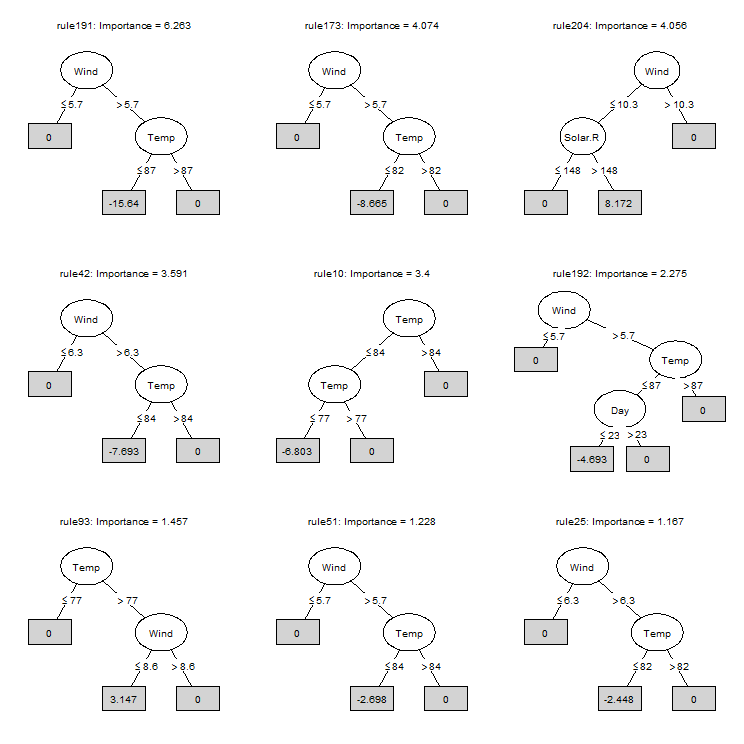
- The package allows for plotting the final rule ensemble as a collection of simple decision trees.
- The initial ensembles may be generated as in bagging, boosting and/or random forests.
- Hinge functions of predictor variables may be included as baselearners, like in the multivariate adaptive regression splines method of Friedman (1991), using the gpe() function.
Note that pre is under development, and much work still needs to be done.
To get a first impression of how pre works, we will fit a prediction rule ensemble to predict Ozone levels using the airquality dataset. We can fit a prediction rule ensemble using the pre() function:
library(pre)
set.seed(42)
airq.ens <- pre(Ozone ~ ., data = airquality[complete.cases(airquality), ])
We can print the resulting ensemble (alternatively, we could use the print method):
airq.ens
#>
#> Final ensemble with cv error within 1se of minimum:
#>   lambda =  2.331694
#>   number of terms = 13
#>   mean cv error (se) = 302.4644 (79.28454)
#>
#>   cv error type : Mean-Squared Error
#>
#>          rule  coefficient                          description
#>   (Intercept)   72.9680699                                 <NA>
#>       rule191  -15.6401488              Wind > 5.7 & Temp <= 87
#>       rule173   -8.6645924              Wind > 5.7 & Temp <= 82
#>       rule204    8.1715564         Wind <= 10.3 & Solar.R > 148
#>        rule42   -7.6928586              Wind > 6.3 & Temp <= 84
#>        rule10   -6.8032890              Temp <= 84 & Temp <= 77
#>       rule192   -4.6926624  Wind > 5.7 & Temp <= 87 & Day <= 23
#>        rule93    3.1468762              Temp > 77 & Wind <= 8.6
#>        rule51   -2.6981570              Wind > 5.7 & Temp <= 84
#>        rule25   -2.4481192              Wind > 6.3 & Temp <= 82
#>        rule28   -2.1119330              Temp <= 84 & Wind > 7.4
#>        rule74   -0.8276940              Wind > 6.9 & Temp <= 84
#>       rule200   -0.4479854                       Solar.R <= 201
#>       rule166   -0.1202175              Wind > 6.9 & Temp <= 82
We can plot the baselarners in the ensemble using the plot method (note that only the nine most important baselearners are requested here):
plot(airq.ens, nterms = 9, cex = .5)We can obtain the estimated coefficients for each of the baselearners using the coef method:
coefs <- coef(airq.ens)
coefs[1:10,]
#>            rule coefficient                         description
#> 201 (Intercept)   72.968070                                <NA>
#> 166     rule191  -15.640149             Wind > 5.7 & Temp <= 87
#> 149     rule173   -8.664592             Wind > 5.7 & Temp <= 82
#> 178     rule204    8.171556        Wind <= 10.3 & Solar.R > 148
#> 39       rule42   -7.692859             Wind > 6.3 & Temp <= 84
#> 10       rule10   -6.803289             Temp <= 84 & Temp <= 77
#> 167     rule192   -4.692662 Wind > 5.7 & Temp <= 87 & Day <= 23
#> 84       rule93    3.146876             Temp > 77 & Wind <= 8.6
#> 48       rule51   -2.698157             Wind > 5.7 & Temp <= 84
#> 23       rule25   -2.448119             Wind > 6.3 & Temp <= 82
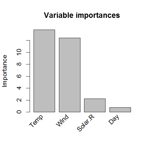
We can assess the importance of input variables as well as baselearners using the importance() function:
importance(airq.ens, round = 4)We can generate predictions for new observations using the predict method:
predict(airq.ens, newdata = airquality[1:4,])
#>        1        2        3        4
#> 31.10390 20.82041 20.82041 21.26840
We can obtain partial dependence plots to assess the effect of single predictor variables on the outcome using the singleplot() function:
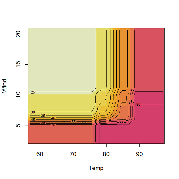
singleplot(airq.ens, varname = "Temp")We can obtain partial dependence plots to assess the effects of pairs of predictor variables on the outcome using the pairplot() function:
pairplot(airq.ens, varnames = c("Temp", "Wind"))
#> Warning in if (!(varnames %in% object$x_names == c(TRUE, TRUE))) {: the
#> condition has length > 1 and only the first element will be used
#> Loading required namespace: akima
#> NOTE: function pairplot uses package 'akima', which has an ACM license. See also https://www.acm.org/publications/policies/software-copyright-notice.
We can assess the expected prediction error of the prediction rule ensemble through cross validation (10-fold, by default) using the cvpre() function:
set.seed(43)
airq.cv <- cvpre(airq.ens)
airq.cv$accuracy
#> $MSE
#>       MSE        se
#> 364.64985  83.83141
#>
#> $MAE
#>      MAE       se
#> 13.75209  1.26322
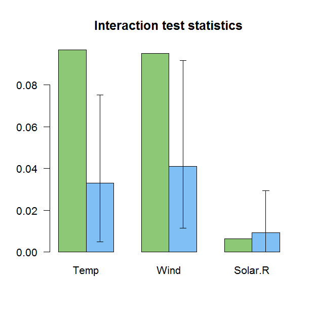
We can assess the presence of input variable interactions using the interact() and bsnullinteract() funtions:
set.seed(44)
nullmods <- bsnullinteract(airq.ens)
int <- interact(airq.ens, nullmods = nullmods, c("Temp", "Wind", "Solar.R"))
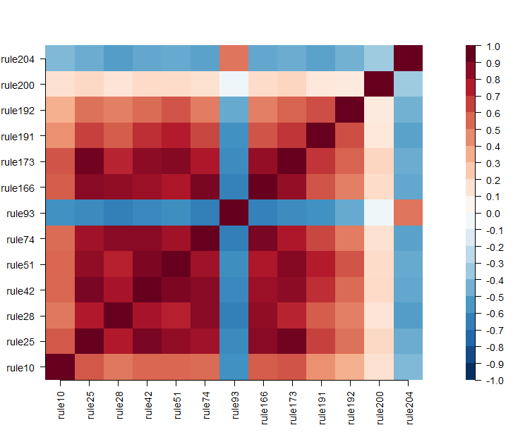
We can check assess correlations between the baselearners using the corplot() function:
corplot(airq.ens)More complex prediction ensembles can be obtained using the gpe() function. The abbreviation gpe stands for generalized prediction ensembles, which may include hinge functions of the predictor variables as described in Friedman (1991), in addition to rules and/or linear terms. Addition of such hinge functions may improve predictive accuracy. More information about fitting generalized prediction ensembles can be obtained by typing:
?gpeFokkema, M. (2017). Pre: An r package for fitting prediction rule ensembles. ArXiv:1707.07149. Retrieved from https://arxiv.org/abs/1707.07149
Friedman, J. H. (1991). Multivariate adaptive regression splines. The Annals of Statistics, 19(1), 1–67.
Friedman, J. H., & Popescu, B. E. (2008). Predictive learning via rule ensembles. The Annals of Applied Statistics, 2(3), 916–954. Retrieved from http://www.jstor.org/stable/30245114
Hothorn, T., Hornik, K., & Zeileis, A. (2006). Unbiased recursive partitioning: A conditional inference framework. Journal of Computational and Graphical Statistics, 15(3), 651–674.
