DeepDrug3D is a tool to predict the protein pocket to be ATP/Heme/other-binding given the binding residue numbers and the protein structure.
If you find this tool useful, please star this repo and cite our paper :)
Pu L, Govindaraj RG, Lemoine JM, Wu HC, Brylinski M (2019) DeepDrug3D: Classification of ligand-binding pockets in proteins with a convolutional neural network. PLOS Computational Biology 15(2): e1006718. https://doi.org/10.1371/journal.pcbi.1006718
This README file is written by Limeng Pu.
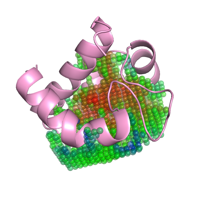
An example of binding grid generated, pdb ID: 1a2sA, atom type: C.ar. Red --> low potentials while Blue --> high potentials.
This is a newer version of the implmentation. Since many people are interested in visualize the output from the grid generation like in the image above, I've decided to seperate the data-generation module and the training/prediction module. Another reason for this iteration of implementation is the dligand-linux used for potential calculation requires 32-bit Linux while Pytorch requires 64-bit Linux. It causes confiliction and resulting in different errors depending on the order you install them. Also the deep learning library used has been changed from Keras to Pytorch.
- System requirement: Linux (DFIRE potential calculation only runs on Linux. Tested on Red Hat Enterprise Linux 6)
- The data-generation module dependencies are provided in
./DataGeneration/environment.yml. Please change line 9 in the file according to your system. To install all the dependencies runconda env create -f environment.yml. - The learning module requires Pytorch. To install it, refer to https://pytorch.org/get-started/locally.
The package provides data-generation, prediction, and training modules.
- Data generation
This module generates data for training/prediction while providing intermediate results for visualization. All files are under ./DataGeneration. The DFIRE potential calculation uses the module (./DataGeneration/dligand-linux) described in A Knowledge-Based Energy Function for Protein−Ligand, Protein−Protein, and Protein−DNA Complexes by Zhang et al. since it is written in Fortran, which is faster than our own implementation in Python.
To generate the binding grid data, run
python voxelization.py --f example.pdb --a example_aux.txt --o results --r 15 --n 31 --p--finput pdb file path.--ainput auxilary file path, with binding residue numbers and center of ligand (optional). An example of the auxilary file is provided inexample_aux.txt.--rthe radius of the spherical grid.--nthe number of points along the dimension of the spherical grid.--ooutput folder path.--por--swhether to calculate the potential nor not. If not, only the binary occupied grid will be returne, i.e., the shape of the grid only. Default, yes (--p).
Several files will be saved, including example_transformed.pdb (coordinate-transformed pdb file), example_transformed.mol2 (coordinate-transformed mol2 file for the calculation of DFIRE potential), example.grid (grid representation of the binding pocket grid for visualization), and example.h5 (numpy array of the voxel representation).
To visualize the output binidng pocket grid, run
python visualization --i example.grid --c 0--iinput binding pocket grid file path.--cchannel to visualize. Note that if you pass--sin the previous step, the channel number--chas to be 0.
An output example_grid.pdb will be generated for visualization. Note this pocket grid matches the transformed protein example_transformed.pdb.
- Prediction
This module classifies the target binding pocket to be either an ATP-, Heme-, or other-type pocket, which basically means which type of ligand it tends to binding to. The trained model is available at https://osf.io/enz69/. All files are under ./Learning.
To use the prediction module, run
python predict.py --f example.h5 --m path_to_the_trianed_model--finput h5 file path.--mpath to the trained model weights.
The output would be something like
The probability of pocket provided binds with ATP ligands: 0.3000
The probability of pocket provided binds with Heme ligands: 0.2000
The probability of pocket provided binds with other ligands: 0.5000
- Training
In order to use our model to train your own dataset, you have to convert your dataset, which will be pdbs to voxel representation of protein-ligand biniding grid representation. The data conversion procedure has been descibed before. The module runs a random 5-fold cross validation. All the related results including loss, accuracy and model weights will be saved. All files are under ./Learning.
The trainig module can be runned as
python train.py --path path_to_your_data_folder --lpath path_to_your_label_file --bs batch_size --lr inital_learning_rate --epoch number_of_epoches --opath output_folder_path--pathpath to the folder contains all the voxel data.--lpathlabel file path. The file should be a comma separated file with no header. The first column is the filename and the second column is the class (starts from 0). An example has been provided./Learning/labels.--bs,--lr,--epochis the hyperparameters related to the model. Recommanded values are 64, 1e-5, 50.--opathIf no output location is provided, alogsfolder will be created under current working directory to store everything.
We provided our dataset we used for the training at https://osf.io/enz69/, which are the voxel representations of ATP, Heme, and other along with the class label file.
