
Implementation of the Nelson-Siegel-Svensson interest rate curve model in Python.
from nelson_siegel_svensson import NelsonSiegelSvenssonCurve
import numpy as np
from matplotlib.pyplot import plot

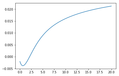
y = NelsonSiegelSvenssonCurve(0.028, -0.03, -0.04, -0.015, 1.1, 4.0)
t = np.linspace(0, 20, 100)
plot(t, y(t))- Free software: MIT license
- Python 3.7 or later supported
- Documentation: https://nelson-siegel-svensson.readthedocs.io.
- Python implementation of the Nelson-Siegel curve (three factors)
- Python implementation of the Nelson-Siegel-Svensson curve (four factors)
- Methods for zero and forward rates (as vectorized functions of time points)
- Methods for the factors (as vectorized function of time points)
- Calibration based on ordinary least squares (OLS) for betas and nonlinear optimization for taus
- Simple command line interface (CLI) for evaluating, calibrating and plotting curves
In order to calibrate a curve to given data you can use the calibrate_ns_ols and calibrate_nss_ols functions in the calibrate module:
import numpy as np
from nelson_siegel_svensson.calibrate import calibrate_ns_ols

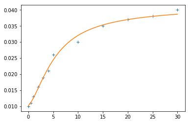
t = np.array([0.0, 0.5, 1.0, 2.0, 3.0, 4.0, 5.0, 10.0, 15.0, 20.0, 25.0, 30.0])
y = np.array([0.01, 0.011, 0.013, 0.016, 0.019, 0.021, 0.026, 0.03, 0.035, 0.037, 0.038, 0.04])

curve, status = calibrate_ns_ols(t, y, tau0=1.0)  # starting value of 1.0 for the optimization of tau
assert status.success
print(curve)
which gives the following output:
NelsonSiegelCurve(beta0=0.04201739383636799, beta1=-0.031829031569430594, beta2=-0.026797319779108236, tau=1.7170972656534174)nelson_siegel_svensson provides basic functionality using a command line interface (CLI):
Usage: nelson_siegel_svensson [OPTIONS] COMMAND [ARGS]...

Commandline interface for nelson_siegel_svensson.

Options:
--help  Show this message and exit.

Commands:
calibrate  Calibrate a curve to the given data points.
evaluate   Evaluate a curve at given points.
plot       Plot a curve at given points.
In order to calibrate a curve to given data points on the command line, try
nelson_siegel_svensson calibrate -t '[0.0, 0.5, 1.0, 2.0, 3.0, 4.0, 5.0, 10.0, 15.0, 20.0, 25.0, 30.0]' -y '[0.01, 0.011, 0.013, 0.016, 0.019, 0.021, 0.026, 0.03, 0.035, 0.037, 0.038, 0.04]' --nelson-siegel --initial-tau1 1.0which gives
{"beta0": 0.042017393764903765, "beta1": -0.03182903146166806, "beta2": -0.026797320316066128, "tau": 1.717097232403383}This curve can then be evaluated on the command line using
nelson_siegel_svensson evaluate -c '{"beta0": 0.042017393764903765, "beta1": -0.03182903146166806, "beta2": -0.026797320316066128, "tau": 1.717097232403383}' -t '[0, 1, 2, 3]'resulting in
[0.010188362303235707, 0.012547870204470839, 0.01574855552855885, 0.01897955804146046]And finally, the curve can be plotted with
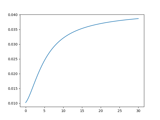
nelson_siegel_svensson plot -o cli_plot_example.png -c '{"beta0": 0.042017393764903765, "beta1": -0.03182903146166806, "beta2": -0.026797320316066128, "tau": 1.717097232403383}'Note that the quoting in the above commands prevents bash from evalutating the JSON-based parameters. Depending on your shell, you may require a different quoting mechanism.
Main developer is luphord.
This package was prepared with Cookiecutter and the audreyr/cookiecutter-pypackage project template.


