MCMC for Forensic Science - Solutions

Questions: https://github.com/rstats-gsoc/gsoc2020/wiki/MCMC-for-forensic-science

Easy

library("seqinr")
fsa_data <- read.abif("A04_RD14-0003-23d3d-0.0078IP-Q2.5_001.5sec.fsa")
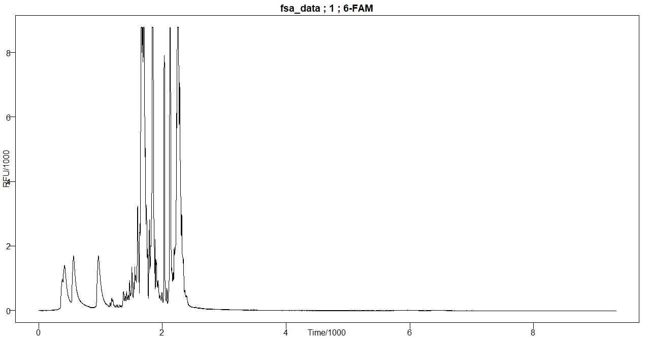
plotabif(fsa_data)

Medium

rm(list=ls())
library("seqinr")
fsa_data <- read.abif("A04_RD14-0003-23d3d-0.0078IP-Q2.5_001.5sec.fsa")
tscale = 1000
tmin = 1/tscale
tmax = fsa_data$Data[["SCAN.1"]]/tscale
irange = (tmin*tscale):(tmax*tscale)
x = irange/tscale

chanel.names = c(1:4,105)

temp <- data.frame()
for(i in 1:5)
{
  chanel = i
  DATA = paste("DATA", chanel.names[chanel], sep = ".")
  yscale = 1000
  y = fsa_data$Data[[DATA]][irange]/yscale
  
  data_label = sapply(rep(DATA, length(fsa_data$Data[[DATA]])), c) # 9335
  
  temp <- rbind(temp, data.frame(x, y, data_label))
}

library(ggplot2)
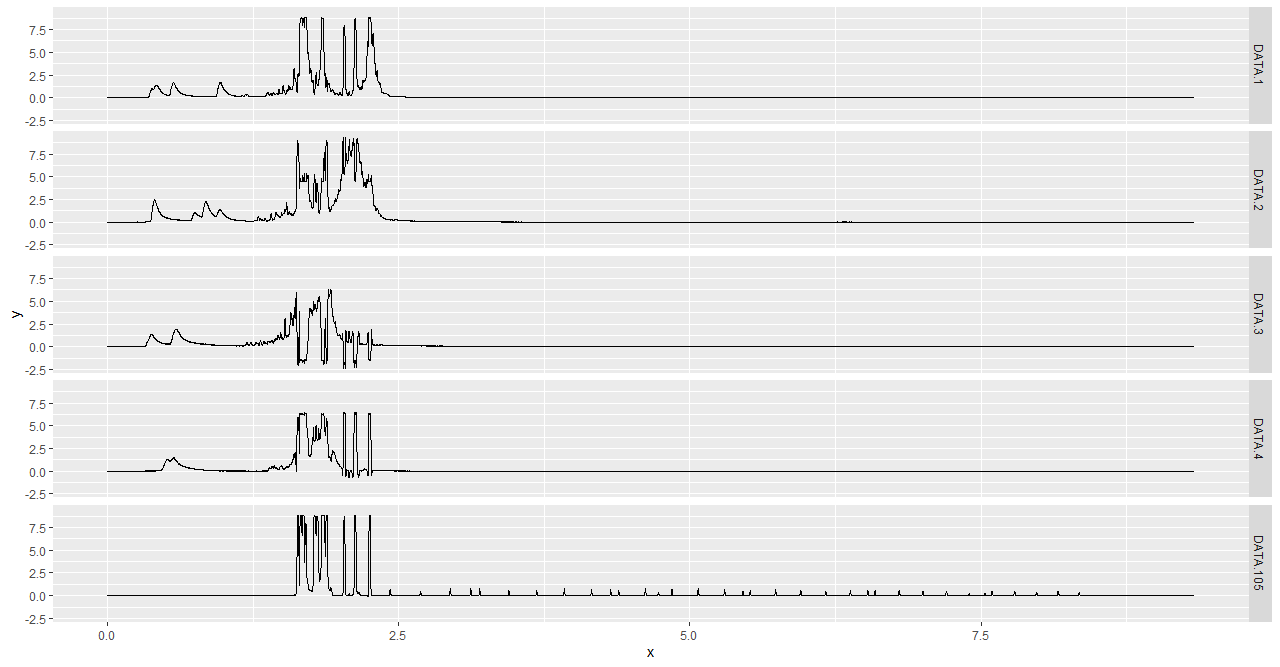
ggplot(temp, aes(x, y)) + geom_line() + facet_grid(data_label~.)

Hard

For the hard problem, I chose to use the rStan package. This package converts models specified in R into Stan model. We start by running a multivariate linear regression on WaffleHouse dataset, where we would estimate the regression coefficient when regressing Divorce on Median age and Marriage rate using lm() function. Then we estimate those coefficients again using rStan given we have a prior knowledge of our problem.

Stan uses Markov chain Monte Carlo(MCMC) to collect samples from the posterior of the regression coefficients. Later we implement MCMC Metropolis-Hastings(MH) algorithm in R to demonstrate the internals of the algorithm. Afterward, we reimplement it in C++ for better performance. Finally we will run benchmark to see the improvement in performance.

Jump to content:

Regression using lm
Regression using rStan
MCMC MH Implementation in R mcmcR
MCMC MH Implementation in Cpp mcmcCpp
Benchmark between mcmcR mcmcCpp

Many supporting codes are omitted from this section of the document for brevity. They are available under the Hard folder.

Regression using lm

Here we are regressing Divorce on Marriage median age and Marriage rate. When using lm function, we are assuming uniform prior distribution on the parameter of interest.

rm(list=ls())
library(rethinking)
data(WaffleDivorce)
d <- WaffleDivorce
d <- d[ , c("Divorce","MedianAgeMarriage","Marriage") ] 

summary(lm(Divorce ~ MedianAgeMarriage + Marriage, data=d))

Here is the summary of the fitted model, and here we can see that the values of the regression coefficient and their standard error. We can see the Median Age is an important predictor in predicting Divorce rate.

Coefficients:
                  Estimate Std. Error t value Pr(>|t|)    
(Intercept)       36.87665    7.66104   4.814 1.58e-05 ***
MedianAgeMarriage -0.99965    0.24593  -4.065 0.000182 ***
Marriage          -0.05686    0.08053  -0.706 0.483594

Regression using rStan

Now, if we have prior knowledge about the parameters, we can encode it in their prior distribution. We can not use lm function anymore since it assumes a uniform prior for the parameters. The new models need to be fit using rStan. We will specify the model with its prior in R and rStan will convert it to a Stan model.

model <- map2stan( 
  alist(
    Divorce ~ dnorm( mu , sigma ) ,
    mu <- a + bA*MedianAgeMarriage + bR*Marriage ,
    a ~ dnorm(0,100),
    bR ~ dnorm(0,10),
    bA ~ dnorm(0,10),
    sigma ~ dcauchy(0,2)
  ) ,
  data=d )
precis(model)

Here is the summary of the fitted model, and we can see that the values of the coefficients are almost equal to our previous analysis. One of the reason they are equal is because our priors have large standard deviation therefore not very strong to sway the estimates.

       mean   sd  5.5% 94.5% n_eff Rhat4
a     37.02 7.53 25.12 48.40   226     1
bR    -0.06 0.08 -0.19  0.07   262     1
bA    -1.00 0.24 -1.38 -0.62   236     1
sigma  1.52 0.16  1.29  1.77   374     1

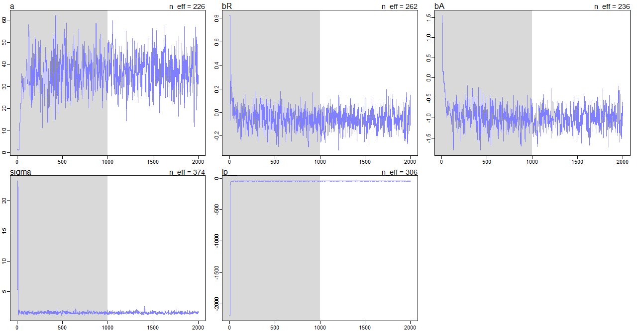
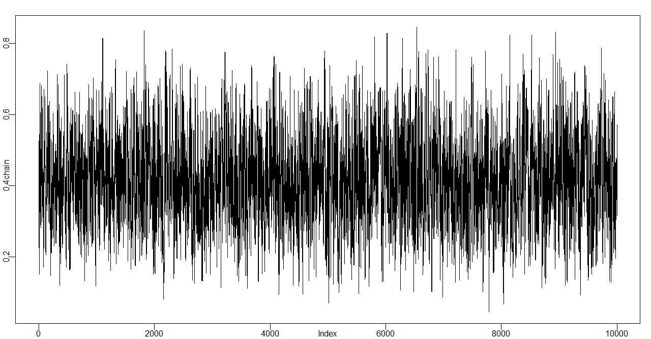
But how Stan is estimating the parameters? It is using the MCMC method. It is a sampling algorithm. To validate the Markon chains generated during the model fitting - we need to check if the chain is stationary. In the following figure, we see that once the parameter values are stationary, which means samples are not deviating too much from the mean results in a stationary Markov chain.

MCMC MH Implementation in R mcmcR

But how does the MCMC sampling works? Here we demonstrate how it works by implementing it in R language.

Given problem: Let's say in a sequence of 10 coin tosses, we get 4 heads. What is the distribution of the probability of head(p) given the event we've just observed?

Here the likelihood function is binomial with a parameter value of 4 and 10. Prior of p follows a beta distribution with 1 and 1 as shape parameters. We need to find the posterior distribution of p given we've observed 4 heads out of 10 coin tosses.

The following function, mcmcR takes 3 parameters. The first one is the number of samples we want to sample from our posterior, the second one is the number of coin tosses results in head, and the final one is the number of trials.

rm(list=ls())
library(raster)

mcmcR <- function(samples, success, trials){
  n <- samples
  chain <- sapply(rep(NA, n), c)
  chain[1] <- 0.5
  lapply(2:n, function(x){
    nextState <- rnorm(1, chain[x-1], sd = 0.16) # Monte Carlo
    
    # estimate probability of head in a coin toss p
    # dbeta(1,1) Almost uniform prior
    # dbinom(4, 10) 4 heads our of 10 tosses
    # Metropolis-Hasting Step
    likelihood_ratio <- 
      (dbeta(nextState,1,1) * dbinom(x=success,size=trials,prob=clamp(nextState,0,1)))/
      (dbeta(chain[x-1],1,1) * dbinom(x=success,size=trials,prob=clamp(chain[x-1],0,1)))
    
    acceptance_prob <- min(likelihood_ratio, 1)
    if(acceptance_prob == 1){
      chain[x]  <<-  nextState
    } else if(acceptance_prob > runif(1)){
      chain[x] <<-  nextState
    } else {
      chain[x]  <<-  chain[x-1]
    }
  })
  return(chain)
}

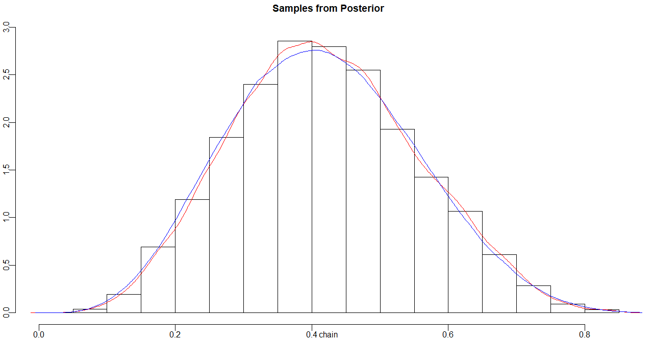
The function returns 10,000 values samples from the posterior. Here we are plotting them in a histogram, and overplotting the kernel density estimate of the same data shown in red. This problem can be solved analytically because of the beta-binomial conjugate. The posterior follows a Beta distribution with 5 and 7 as a shape parameter, which is shown in Blue. Since the blue and red distribution is almost similar - we conclude that our estimation is correct. Here we can also see that the mode is estimating the mean for p is about 0.4, which is 4 heads out of 10 tosses.

Here we are checking that Markov chain(samples) are stationary, and since the values do not seem to deviate too much from the mean, we conclude that the chain is stationary.

MCMC MH Implementation in Cpp mcmcCpp

R is known to be slow because it lacks fine-grained control over memory. So we reimplement the same algorithm in C++. Afterward, we test the difference in performance.

Here is the C++ implementation of the MCMC HM algorithm that is available in MCMCHMSampler package available inside the Hard directory.

#include <Rcpp.h>
#include <cmath>
using namespace Rcpp;

// [[Rcpp::export]]
NumericVector mcmcCpp(int length, int success, int trials) {
  NumericVector chain(length);
  
  chain[0] = 0.5;

  for(int x = 1; x<length; x++){
    double nextState = rnorm(1, chain[x-1], 0.16)[0];

    double numvalue = nextState;
    numvalue = numvalue<0.001?0.001:numvalue;
    numvalue = numvalue>0.999?0.999:numvalue;

    double numerator = R::dbeta(nextState, 1, 1, false) * R::dbinom(success, trials, numvalue, false);
    double denumerator = R::dbeta(chain[x-1], 1, 1, false) * R::dbinom(success, trials, chain[x-1], false);
    double likelihood_ratio = numerator / denumerator;
    
    double acceptance_prob = std::min(1.0, likelihood_ratio);
    if( acceptance_prob == 1.0){
      chain[x] = nextState;
    }else if(acceptance_prob > Rcpp::runif(1)[0]){
      chain[x] = nextState;
    }else{
      chain[x] = chain[x-1];
    }
  }
  return chain;
}

Once we've installed the library locally, we can call the implementation from R in the following manner.

chainCpp <- mcmcCpp(10000, 4, 10)
plot(chainCpp, type="l")

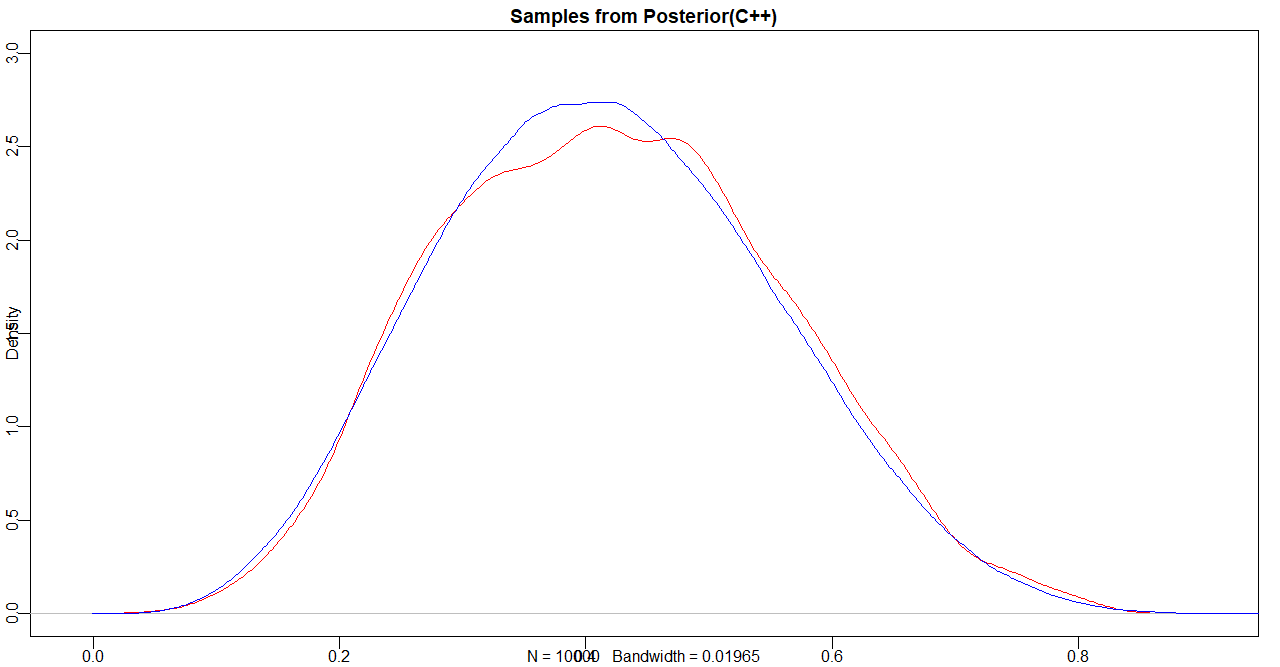
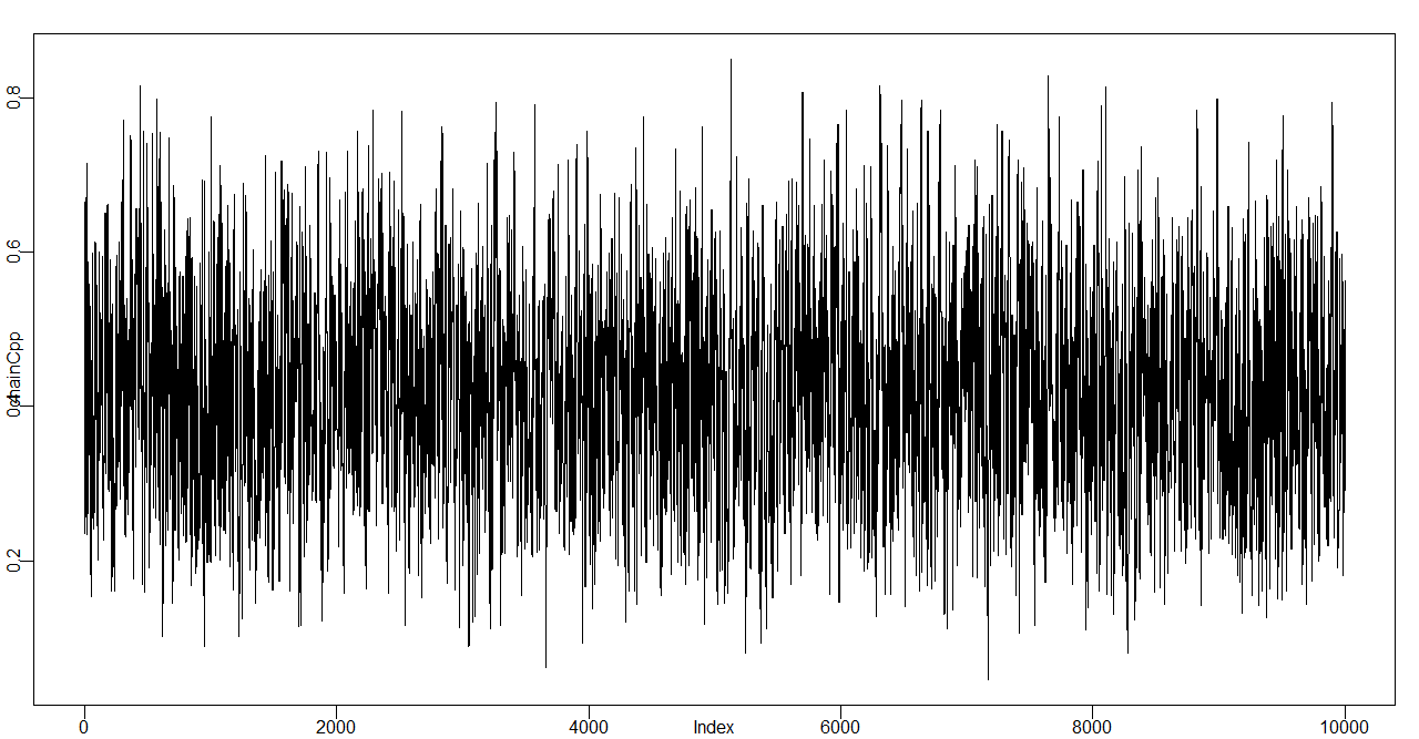
Similar to the last section, we can look at the distribution of the sample, which is marked in red, and it closely follows the analytic solution, which is marked in blue. From the trace plot, we see that the chain is stationary.

Benchmark between mcmcR mcmcCpp

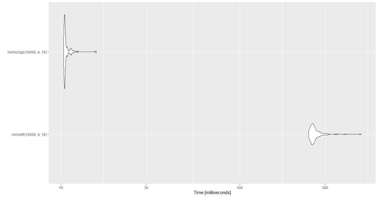
Lets look at the performance difference between this two implementation using microbenchmark R package. Here we can see that the C++ implementation is outperforming the R implementation even when the algorithm was implementated as-is.

library(microbenchmark)
library(ggplot2)
benchmark_result <- microbenchmark(mcmcR(10000, 4, 10), mcmcCpp(10000, 4, 10))
ggplot2::autoplot(benchmark_result)

The mean elapsed time for mcmcCpp is 10 milliseconds and 264 milliseconds for mcmcR. The C++ implementation is about 25 times faster than R implementation.

quazi-irfan/R-Language-Google-Summer-of-Code-Application-2020