landscapetools provides utility functions to work with landscape data
(raster* Objects).
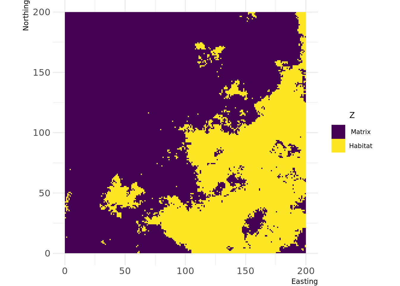
util_binarize: Binarize continuous raster values, if > 1 breaks are
given, return a RasterBrick.
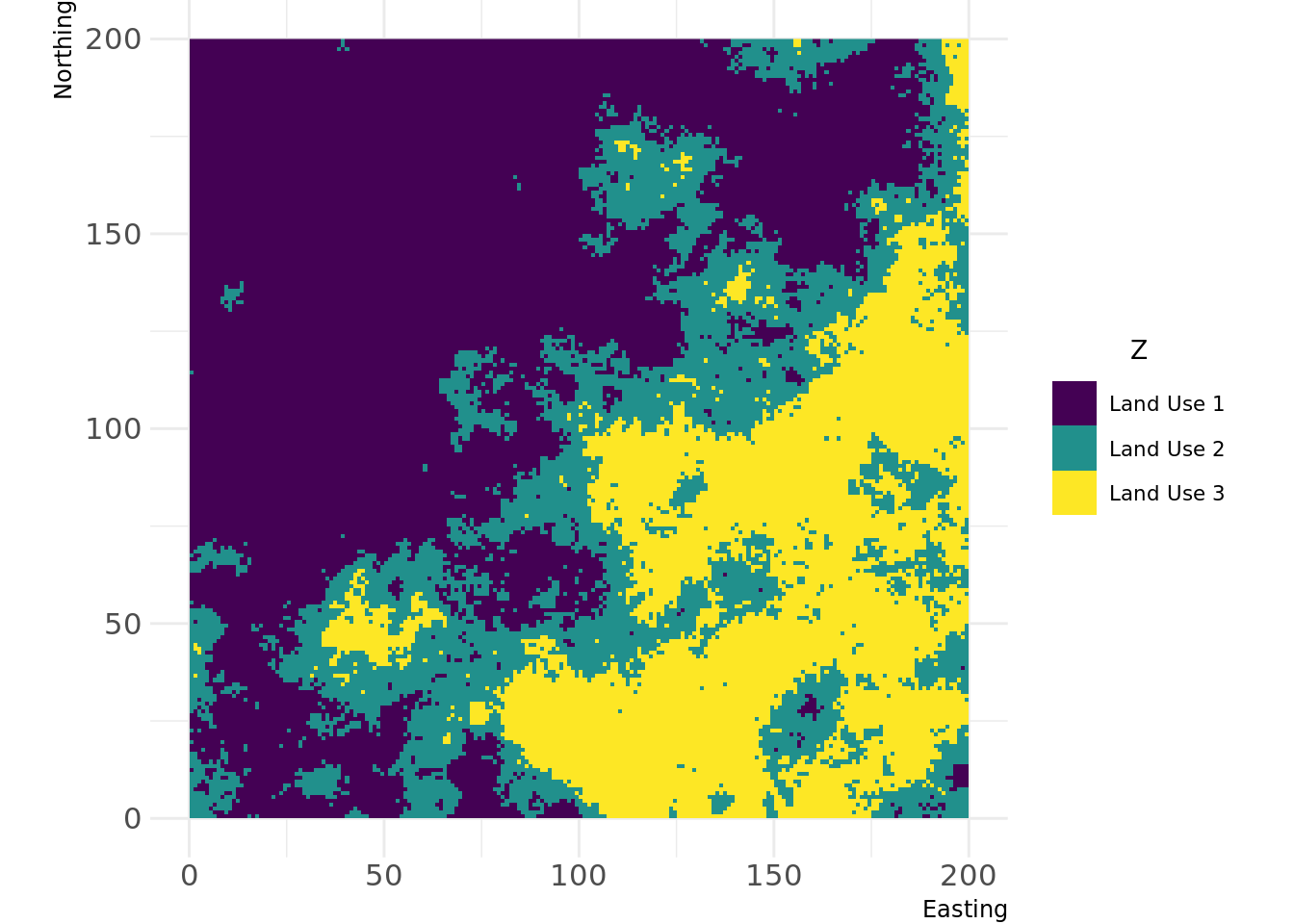
util_classify: Classify a raster
into proportions based upon a vector of class weightings.
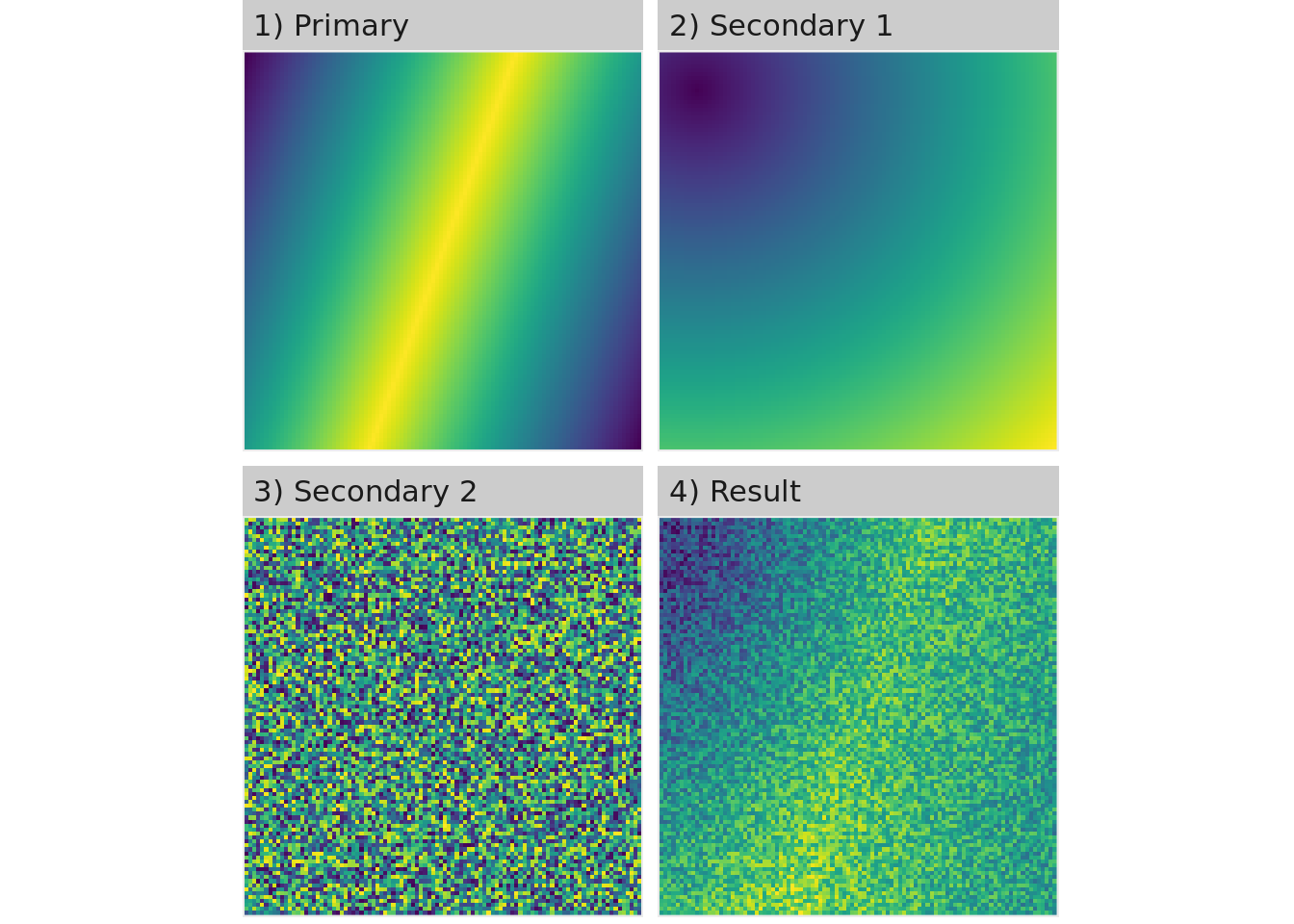
util_merge: Merge a primary raster with other rasters weighted by
scaling factors.
util_raster2tibble, util_tibble2raster: Coerce
raster* objects to tibbles and vice versa.
util_rescale:
Linearly rescale element values in a raster to a range between 0 and
1.
util_plot: Plot a Raster* object with the landscapetools default
theme (as ggplot).
util_facetplot: Plot multiple raster
(RasterStack, -brick or list of raster) side by side as facets.
theme_nlm, theme_nlm_grey: Opinionated ggplot2 theme to visualize
raster (continuous data).
theme_nlm_discrete,
theme_nlm_grey_discrete: Opinionated ggplot2 theme to visualize raster
(discrete data).
theme_faceplot: Opinionated ggplot2 theme to
visualize raster in a facet wrap.
util_import_roboto_condensed:
Import Roboto Condensed font for theme_nlm.
You can install the development version from GitHub with:
# install.packages("devtools")
devtools::install_github("ropensci/landscapetools", ref = "develop")library(NLMR)
library(landscapetools)
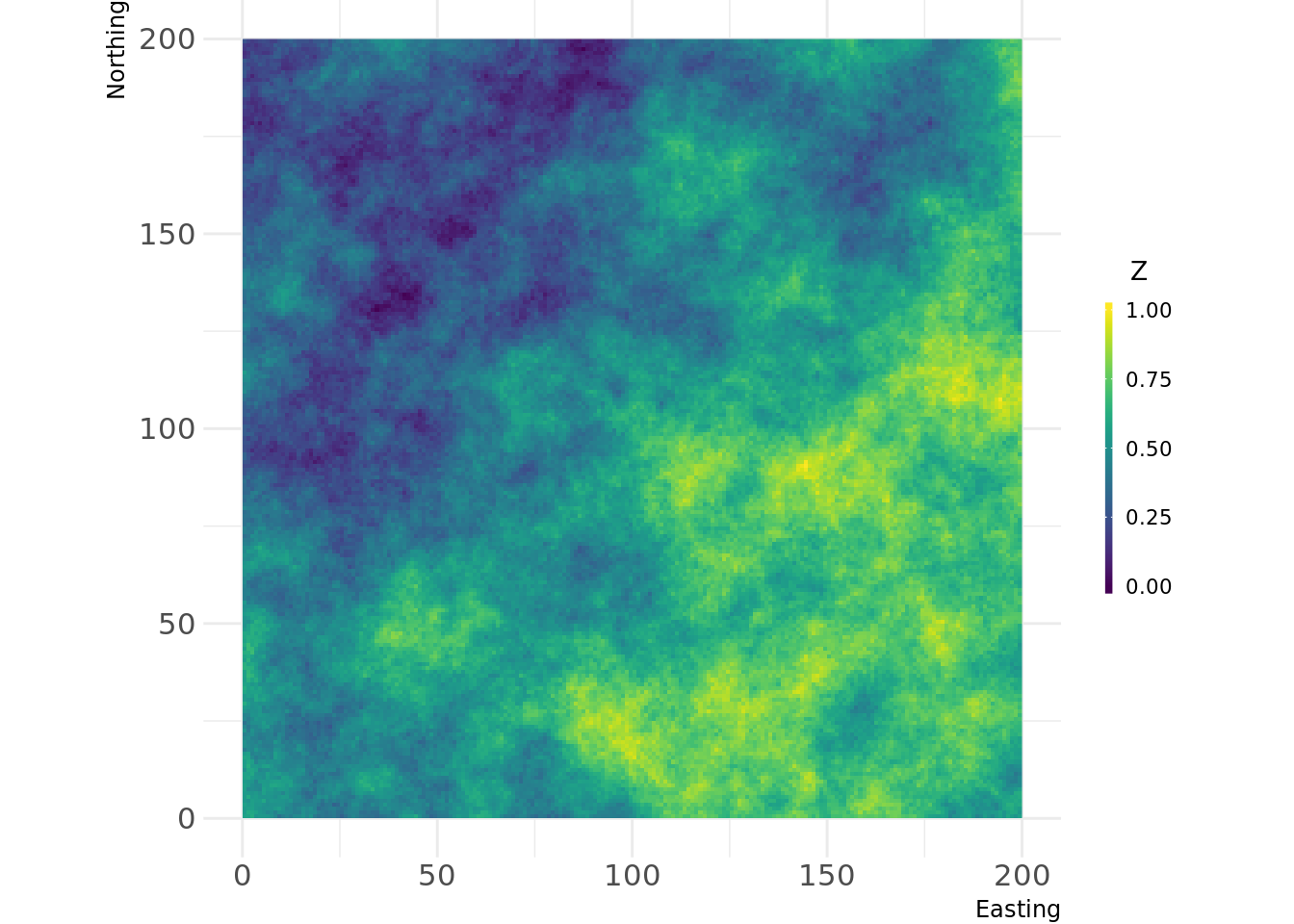
# Create an artificial landscape
nlm_raster <- nlm_fbm(ncol = 200, nrow = 200, fract_dim = 0.8)
util_plot(nlm_raster)# Binarize the map into habitat and matrix
binarized_raster <- util_binarize(nlm_raster, breaks = 0.31415)
util_plot(binarized_raster, discrete = TRUE)# Classify the map into land uses
classified_raster <- util_classify(nlm_raster,
c(0.5, 0.25, 0.25),
level_names = c("Land Use 1", "Land Use 2", "Land Use 3"))
util_plot(classified_raster, discrete = TRUE)# Create a primary and two secondary maps
prim <- nlm_edgegradient(ncol = 100, nrow = 100)
sec1 <- nlm_distancegradient(ncol = 100, nrow = 100,
origin = c(10, 10, 10, 10))
sec2 <- nlm_random(ncol = 100, nrow = 100)
# Merge all maps into one
merg <- util_merge(prim, c(sec1, sec2), scalingfactor = 1)
# Plot an overview
merge_vis <- list(
"1) Primary" = prim,
"2) Secondary 1" = sec1,
"3) Secondary 2" = sec2,
"4) Result" = merg
)
util_facetplot(merge_vis)In the examples above we make heavy use of the NLMR package. Both
packages were developed together until we split them into pure landscape
functionality and utility tools. If you are interested in generating
neutral landscapes via a multitude of available algorithms take a closer
look at the NLMR package.
- Please report any issues or bugs.
- License: GPL3
- Get citation information for
landscapetoolsin R doingcitation(package = 'landscapetools') - We are very open to contributions - if you are interested check
Contributing.
- Please note that this project is released with a Contributor Code of Conduct. By participating in this project you agree to abide by its terms.


