This research was conducted between 1st November 2019 and 22nd January 2020 by Alexandros Kornilakis (University of Crete, FORTH-ICS institute) and Andrew Patel (F-Secure Corporation) as part of EU Horizon 2020 projects PROTASIS and SHERPA, and F-Secure's Project Blackfin. SHERPA is an EU-funded project which analyses how AI and big data analytics impact ethics and human rights. PROTASIS is a project that aims to expand the reach of systems security to the international community via joint research efforts. The PROTASIS project has received funding from the European Union’s Horizon 2020 research and innovation programme under the Marie Skłodowska-Curie grant agreement, No. 690972. Project Blackfin is a multi-year research effort aimed at investigating how to apply collective intelligence in the cyber security domain.
Due to the complex nature of human language, automated detection of negativity and toxicity in content posted on forums, comments sections, and social networks is a difficult task. We posit that an accurate method to cluster textual content is a necessary precursor to any system that may eventually be capable of detecting abusive content, especially on platforms that limit the length of messages that can be authored (such as Twitter). Clustering can be used to find similar phrases, such as those found in regular spam, reply-spam-based propaganda, and content artificially amplified by organized disinformation groups. It is also useful for identifying topics of conversation (what people think about something or someone, what people are talking about), and may also be used to measure sentiment around those topics (how strongly people agree or disagree with something or someone). As this article will illustrate, accurate clustering can also be used to identify other interesting phenomena, such as users who attempt to "hide" spam by slightly altering each of their tweets, groups of accounts spreading hatred towards specific demographics, and groups of accounts spreading disinformation, hoaxes, and fake news.
In this article, we detail our own novel clustering methodology, based on meta embeddings and community detection, and the results of applying that methodology a number of different datasets collected from Twitter, including replies to US politicians, tweets captured against hashtags pertaining to the 2019 UK general elections, and content gathered from UK far-right activists. We present several examples of the output of our clustering methodology, including analysis and interpretation of the results we obtained, and an interactive site for readers to explore. We also discuss some future directions for this line of research. To the best of our knowledge, our approach is the most sophisticated method to date for clustering tweets.
Anyone who's read comments sections on news sites, looked at replies to social media posts authored by politicians, or read comments on YouTube will appreciate that there's a great deal of toxicity on the internet. Some female and minority high-profile Twitter users are the target of constant, serious harassment, including death threats (https://www.youtube.com/watch?v=A3MopLxgvLc) from both individuals and coordinated groups of users. Social media posts authored by politicians, journalists, and news organizations often receive large numbers of angry or downright toxic replies from people who don't support their statements or opinions. Some of these replies originate from fake accounts that have been created for the express purpose of trolling - the process of posting controversial comments designed to provoke emotional reactions and start fights. Trolling is a highly efficient way to spread rumors and disinformation, alter public opinion, and disrupt otherwise meaningful conversation, and, as such, is a tool often used by organized groups of political activists, commercial troll farms, and nation state disinformation campaigns.
On Twitter, troll accounts sometimes use a technique called reply-spamming to fish for engagement. This technique involves replying to a large number of high-profile accounts with the same or similar messages. This achieves two goals. The first is organic visibility - many people read replies to posts from politicians, and thus may read the post from the troll account. The second is social engineering – people get angry and reply to the troll’s posts, and occasionally the owner of the high-profile account may be tricked into engaging with the post themselves. Although high-profile accounts are rarely engaged by such tactics, it's not unheard of.
The problem of analyzing and detecting abuse, toxicity, and hate speech in online social networks has been widely studied by the academic community. Recent studies made use of word embeddings to recognise and classify hate speech on Twitter (https://arxiv.org/pdf/1809.10644.pdf, https://arxiv.org/pdf/1906.03829.pdf), and Chakrabarty et. al. have used LSTMs to visualize abusive content on Twitter, by highlighting offensive use of language (https://arxiv.org/pdf/1809.08726.pdf).
The challenges involved in detecting online abuse are discussed in a paper published by the Alan Turing Institute (https://www.turing.ac.uk/sites/default/files/2019-07/vidgen-alw2019.pdf) Furthemore, issues surrounding the detection of cyber-bullying and toxicity are discussed by Tsapatsoulis et. al (https://encase.socialcomputing.eu/wp-content/uploads/2019/05/NicolasTsapatsoulis.pdf). An approach for detecting bullying and aggression on twitter is proposed by Chatzakou et. al at (https://arxiv.org/pdf/1702.06877.pdf). Srivastava et. al have used capsule networks to identify toxic comments (https://www.aclweb.org/anthology/W18-4412.pdf). The challenges of classifying toxic comments are discussed further by van Aken et. al (https://arxiv.org/pdf/1809.07572.pdf).
We note that methods involving the use of word embeddings have been previously used to cluster Twitter textual data (https://ieeexplore.ieee.org/document/7925400), and that community detection has been applied to text classification problems (https://arxiv.org/abs/1909.11706). However, we have not encountered literature referencing the combination of both. To the best of our knowledge, our approach is the most sophisticated method to date for clustering tweets.
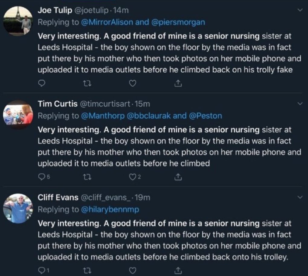
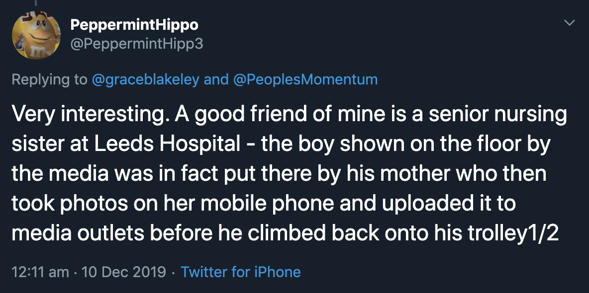
Reply-spam was also used to successfully propagate disinformation during the run-up to the December 2019 UK general election. One such occasion involved a situation where a journalist attempted to show a picture of a child sleeping on the floor of an overcrowded hospital to Boris Johnson during a television interview. Instead of looking at the picture, Johnson pocketed the reporter's phone and attempted to change the subject of their conversation. A clip of the interview went viral on social media, and shortly after, a large number of accounts published posts on various social networks, including Facebook and Twitter, claiming to be an acquaintance of one of the senior nurses at the hospital, and that the aforementioned nurse could verify that the picture was faked (https://twitter.com/marcowenjones/status/1204183081009262592).
Above: some of the original reply spam tweets regarding the Leeds Hospital incident. Note how they are all replies to politicians and journalists.
Above: tory activists on Twitter reinforced the original campaign with more copy-paste reply spam
Above: this was shortly followed by a second campaign containing a different tweet that was also copy-pasted across social networks (by the same group of tory activists)
Many of the accounts that posted this content on Twitter were created specifically for that purpose, and deleted shortly afterwards (https://twitter.com/r0zetta/status/1204519439640801280). The picture of the child sleeping on the floor of the hospital had appeared a week prior to the interview with Johnson in a local newspaper, and at that time, both the story and picture had been verified with personnel at the hospital. However, the fake social media posts were amplified to such a degree that voters, including those living in Leeds, believed that the picture had been faked. At least on Twitter, this disinformation was spread using reply-spam aimed at posts authored by politicians and journalists.
During the run-up to the 2019 UK general elections, posts on social networks were enough to propagate false information. Very few traditional "fake news" sites were uncovered, and it is unlikely that those that were found had any significant impact. Fake news sites are traditionally created in order to give legitimacy to fabricated, "clickbait" headlines. However, people are often inclined to share a headline without even visiting the original article. As such, fake news sites are rarely necessary. Nowadays, it is often enough to simply post something emotionally appealing on a social network, promote it enough to reach a handful of people, and then sit back and watch as it is organically disseminated by proxy. Once a rumor or lie has been spread in this manner, it enters the public’s consciousness, and can be difficult to later refute, even if the initial claim is debunked (https://twitter.com/r0zetta/status/1210499949064052737).
Anyone who runs a prominent social media account is unlikely to be able to find relevant or interesting replies to content they've posted due to the fact that they must wade through hundreds or even thousands of replies, many of which are toxic. This essentially amounts to an informational denial of service for both the account owner, and anyone with a genuine need to contact them. Well-established anti-spam systems exist to assist users with this problem for email, but no such systems exist for social networks. Since notification interfaces on most social networks don't scale well for highly engaged accounts, an automated filtering system would be a more than welcome feature.
Detection of unwanted textual content such as email spam and hate speech is a much easier task than detecting nuances in language indicative of negativity or toxicity. Spam messages typically follow patterns that can be accurately separated with clustering techniques or even regular expressions. Hate speech often contains words that are rarely used outside of their context, and hence can be successfully detected with string matches and other relatively simple techniques. One might assume that sentiment analysis techniques could be used to find toxic content, but they are, unfortunately, still rather inaccurate on real-world data. They often fail to understand the fact that the context of a word can drastically alter its meaning (e.g. "You're a rotten crook" versus "You’ll beat that crook in the next election"). Although accurate sentiment analysis techniques may eventually be of use in this area, software designed to filter toxic comments may require more metadata (such as the subject matter, or topic of the message) in order to perform accurately, or to provide a better explanation as to why certain messages were filtered.
In the context of our work, clustering (or topic modelling) is the process of grouping phrases or passages (or, in this case, tweets) into "buckets" based on their topic or subject matter. Clustering of textual content is useful for finding similar phrases, such as those found in regular spam (e.g. porn bots), reply-spam-based propaganda, and content artificially amplified by organized disinformation groups. It is also useful for identifying topics of conversation (what people think about something or someone, what people are talking about), and may also be used to measure sentiment around those topics (how strongly people agree or disagree with something or someone). As this article will illustrate, accurate clustering can also be used to identify other interesting phenomena, such as users who attempt to "hide" spam by slightly altering each of their tweets (something that is cumbersome to detect via regular expressions), groups of accounts spreading hatred towards specific demographics, and groups of accounts spreading disinformation, hoaxes, and fake news. Furthermore, the results of accurate clustering and topic modeling can be fed into downstream tasks such as:
-
systems designed to fact-check posts and comments
-
systems designed to detect and track rumors and the spread of disinformation, hoaxes, scams, and fake news
-
systems designed to identify the political stance of content published by one or more accounts or conversations
-
systems designed to quantify public opinion and assess the impact of social media on public opinion
-
trust analysis tasks (including those used to determine the quality of accounts on social networks)
-
the creation of disinformation knowledge bases and datasets
-
detection of bots or spam publishers
To this end, we have attempted to build a system that is capable of clustering the type of written content typically encountered on social networks (or more specifically, on Twitter). Our experiments focus on tweets posted in reply to content authored by prominent US politicians and presidential candidates.
We started by collecting two datasets:
The first set captured direct replies to tweets published by a number of highly engaged democrat-affiliated Twitter accounts - @JoeBiden, @SenSanders, @BernieSanders, @SenWarren, @ewarren, @PeteButtigieg, @MikeBloomberg, @amyklobuchar, @AndrewYang and @AOC - between Sun Dec 15 2019 and Mon Jan 13 2020. A total of 978,721 tweets were collected during this period. After preprocessing, a total of 719,617 tweets remained.
The second set captured direct replies to tweets published by @realDonaldTrump between Sun Dec 15 2019 and Wed Jan 08 2020. A total of 4,940,317 tweets were collected during this period. Due to the discrepancy between the sizes of the two collected datasets, we opted to utilize a portion of this set containing 1,022,824 tweets. After preprocessing, a total of 747,232 tweets remained.
We developed our own clustering methodology for this research, which involved preprocessing of captured data, converting tweets into sentence vectors (using different techniques), combining those vectors into meta embeddings, and then creating node-edge graphs using similarities between calculated meta embeddings. Clusters were then derived by performing community detection on the resulting graphs. A detailed description of our methodology can be found in appendix 1 of this article.
Our first experiment involved clustering of a subset of data in set 1 (US democrats). We clustered a batch of 34,003 tweets, resulting in 209 clusters. We created an interactive demo using results of this clustering experiment (https://twitter-clustering.web.app/). Note that this interactive demo will not display correctly on mobile browsers, so we encourage you to visit it from a desktop computer. Use the scroll wheel to zoom in and out of the visualization space, left-click and drag to move the nodes around, and click on nodes or communities themselves to see details. Details include names of accounts that were replied to the most in tweets assigned to that cluster, subject-verb-object triplets and overall sentiment extracted from those tweets, and the two most relevant tweets, loaded on the right of the screen, as examples. Different communities related to different topics (e.g. Community 2 contains clusters relevant to recent events in Iran).
The image below is a static graph visualization of the discovered clusters. Labels were derived by matching commonly occurring words, and bigram combinations of those words, with ngrams and subject-verb-object triplets found in the tweets contained within each cluster. The code for doing this can be found in our github repo (https://github.com/r0zetta/meta_embedding_clustering).
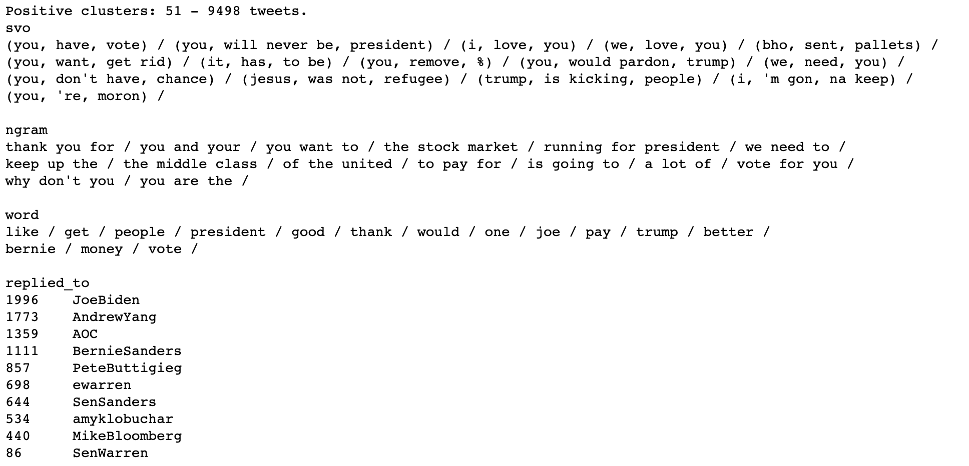
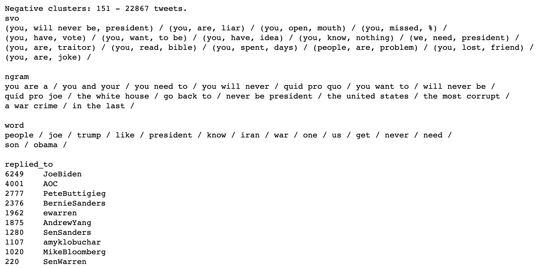
We ran sentiment analysis on each cluster by taking the average sentiment calculated across all tweets contained in the cluster. Sentiment analysis was performed with TextBlob’s lexical sentiment analyzer. We then summarized negative and positive groups of clusters by counting words, ngrams, and which account was replied to. We also extracted subject-verb-object triplets from clusters using the textacy python module.
Note how, in the above, sentiment analysis has incorrectly categorized a few statements such as “you will never be president” and "you're a moron" as positive.
As you can see in the above, negative clusters outnumbered positive clusters by a factor of two.
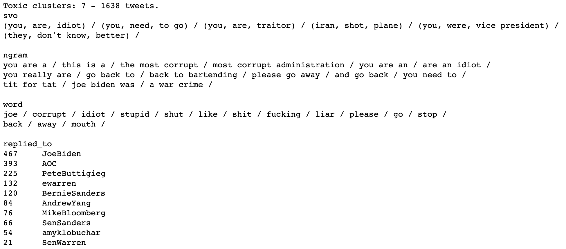
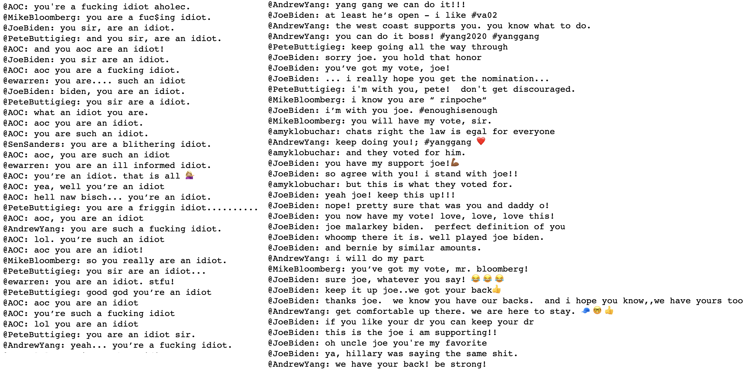
Above are clusters designated toxic by virtue of their average sentiment score. Negative posts are defined as those that express disagreement with the author; toxic posts are more strongly worded and tend to express hostility or downright hatred.
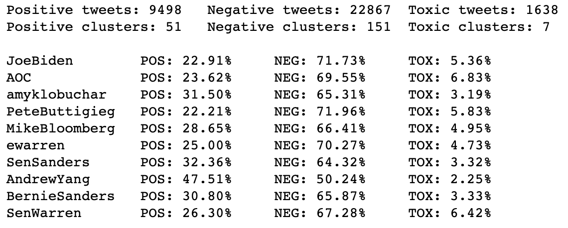
Above is a breakdown of replies by verdict for each candidate. Percentage-wise, @AndrewYang received by far the most positive replies, and @AOC and @SenWarren received the largest ratio of toxic replies.
This simple analysis isn’t, unfortunately, all that accurate, due to deficiencies in the sentiment analysis library used.
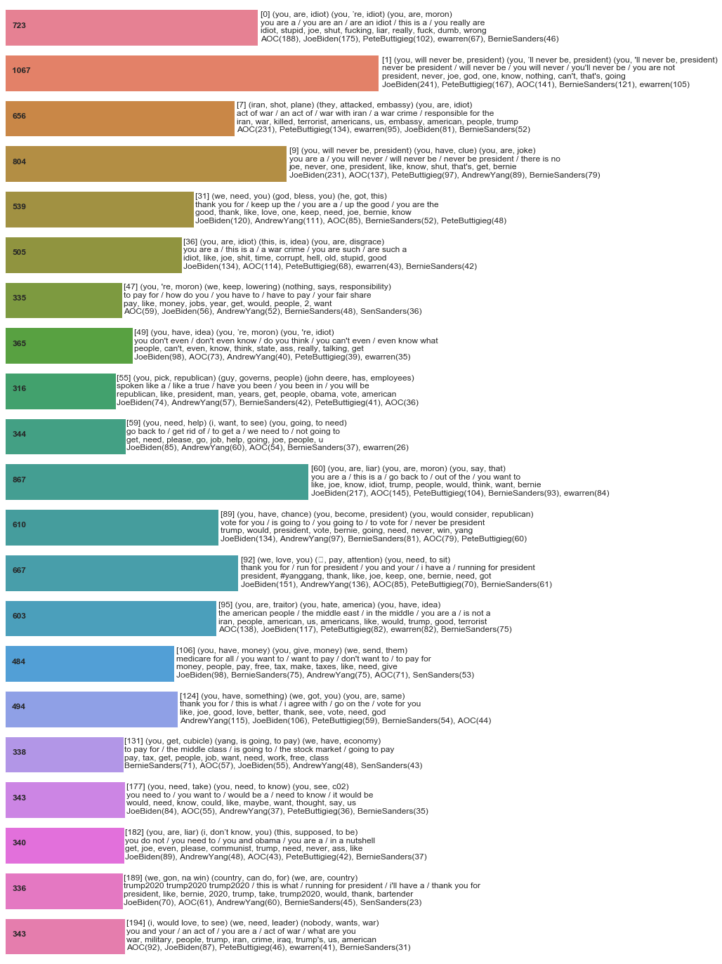
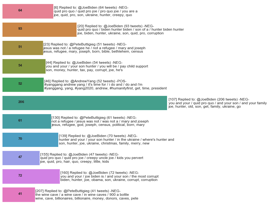
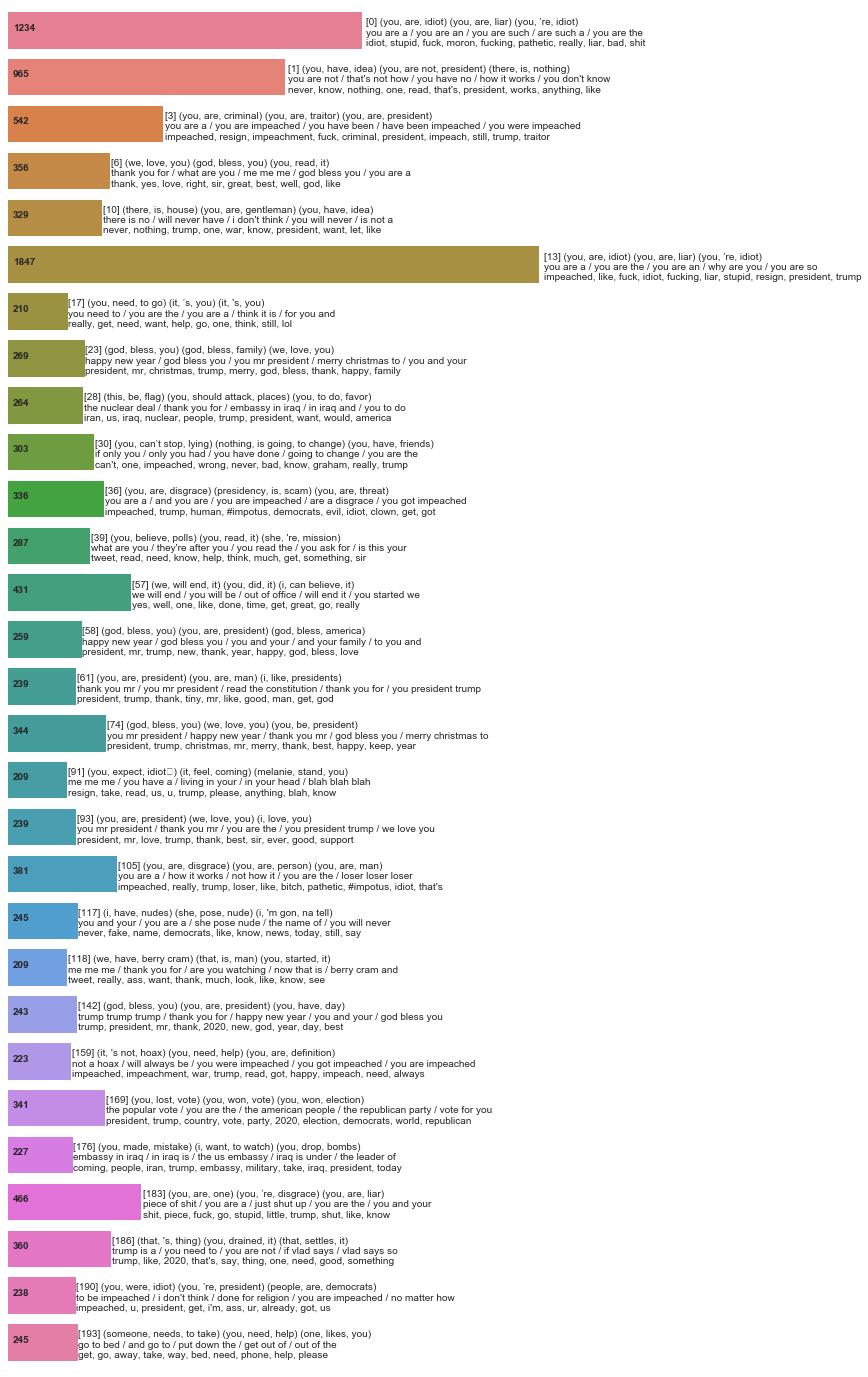
The following chart contains summaries of some of the larger clusters identified. Most of the larger clusters contained negative replies, including common themes such as:
-
you are an idiot/moron/liar/traitor (or similar)
-
you will never be president
-
Trump will win the next election
Positive themes included:
-
We love you
-
You got this
-
You have my vote
Several clusters contained replies directed at just one account. They contained either replies to specific content posted by that account, or comments specifically directed at the politician’s history or personal life, including the following:
-
Comments about Joe Biden’s son
-
Replies to Pete Buttigieg correcting him on a tweet about Jesus being a refugee
-
Comments about Joe Biden’s involvement in the Ukraine
-
Comments about Pete Buttigieg’s net worth, and something about expensive wine
-
Highly positive replies to Andrew Yang’s posts
Above: two discovered clusters – one containing toxic replies, and another containing praise
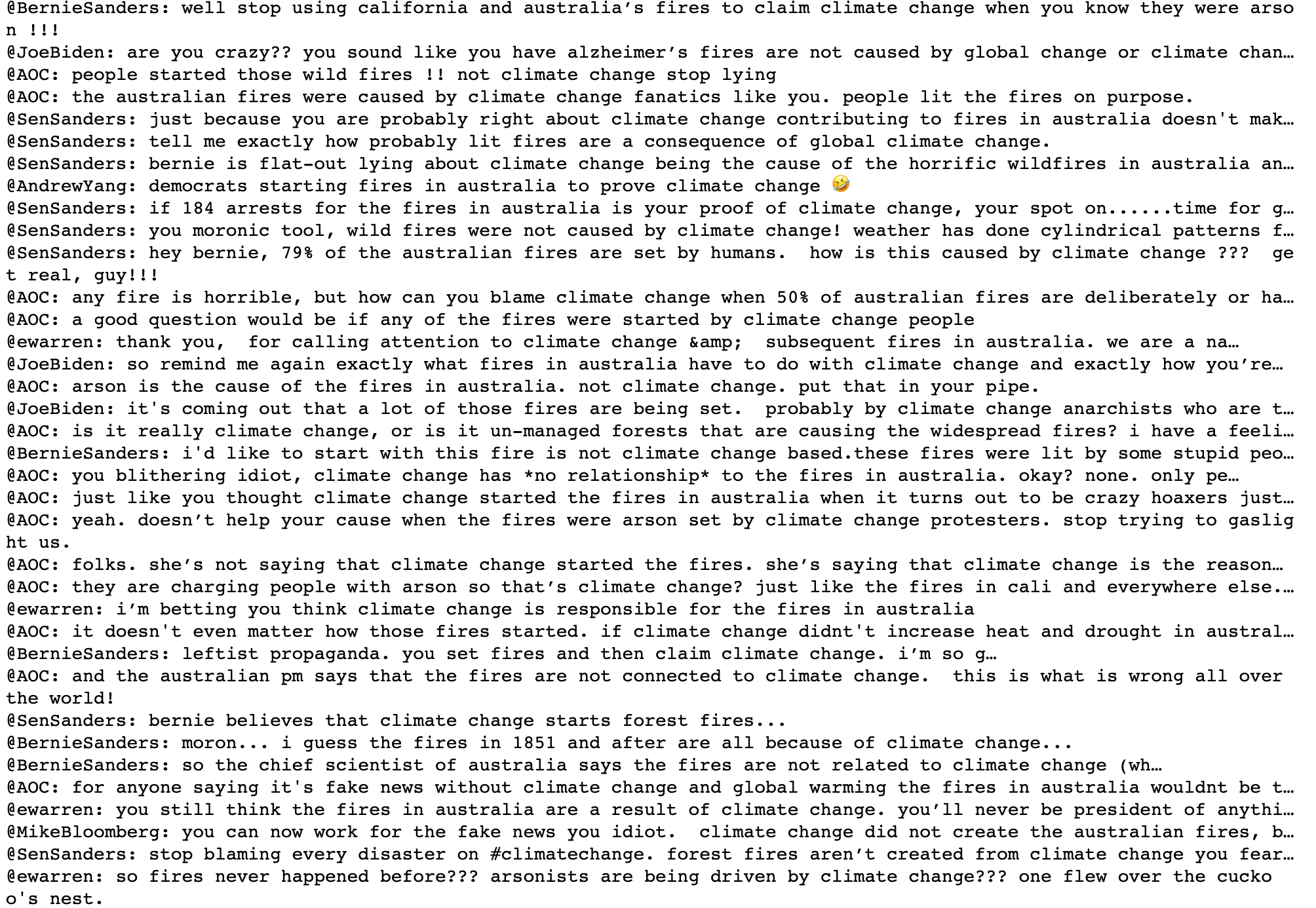
The above discovered cluster contains accounts propagating a hoax that the 2019 bushfires in Australia were caused by arsonists
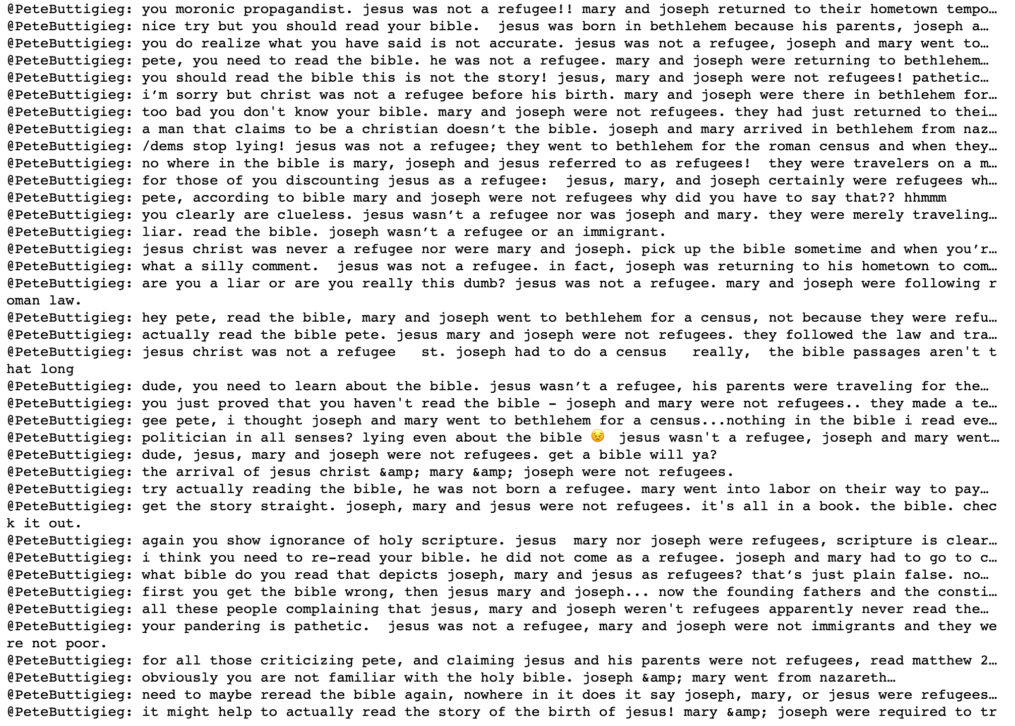
Above is one of a few clusters containing replies only to Pete Buttigieg, where Twitter users state that Jesus wasn’t a refugee
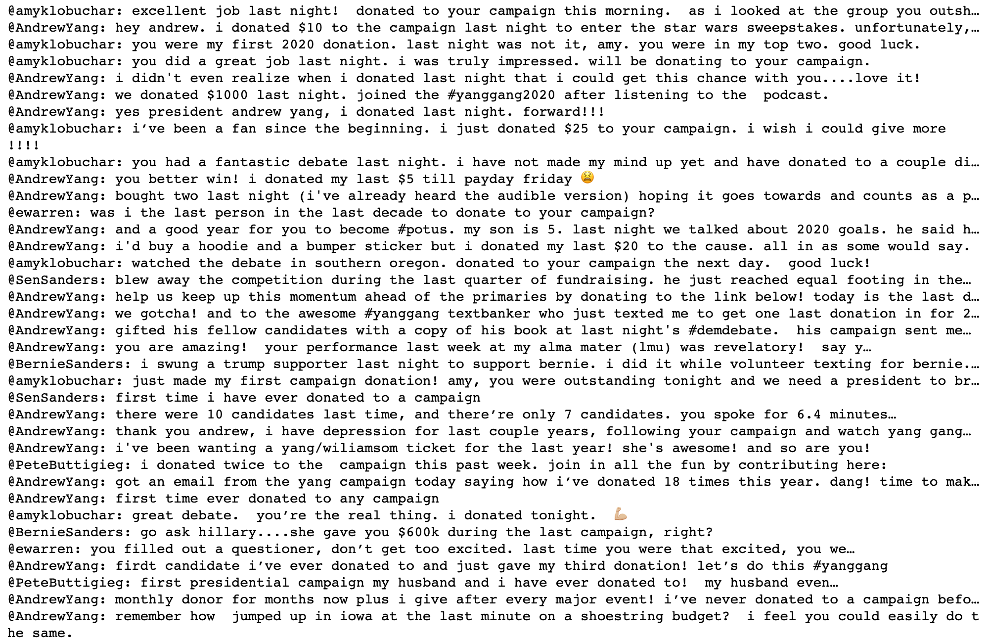
The cluster shown above contains positive comments to democratic presidential candidates that were posted after a debate
Example output from this dataset can be found in our github repo (https://github.com/r0zetta/meta_embedding_clustering/blob/master/example_output/tweet_graph_analysis_dems.txt).
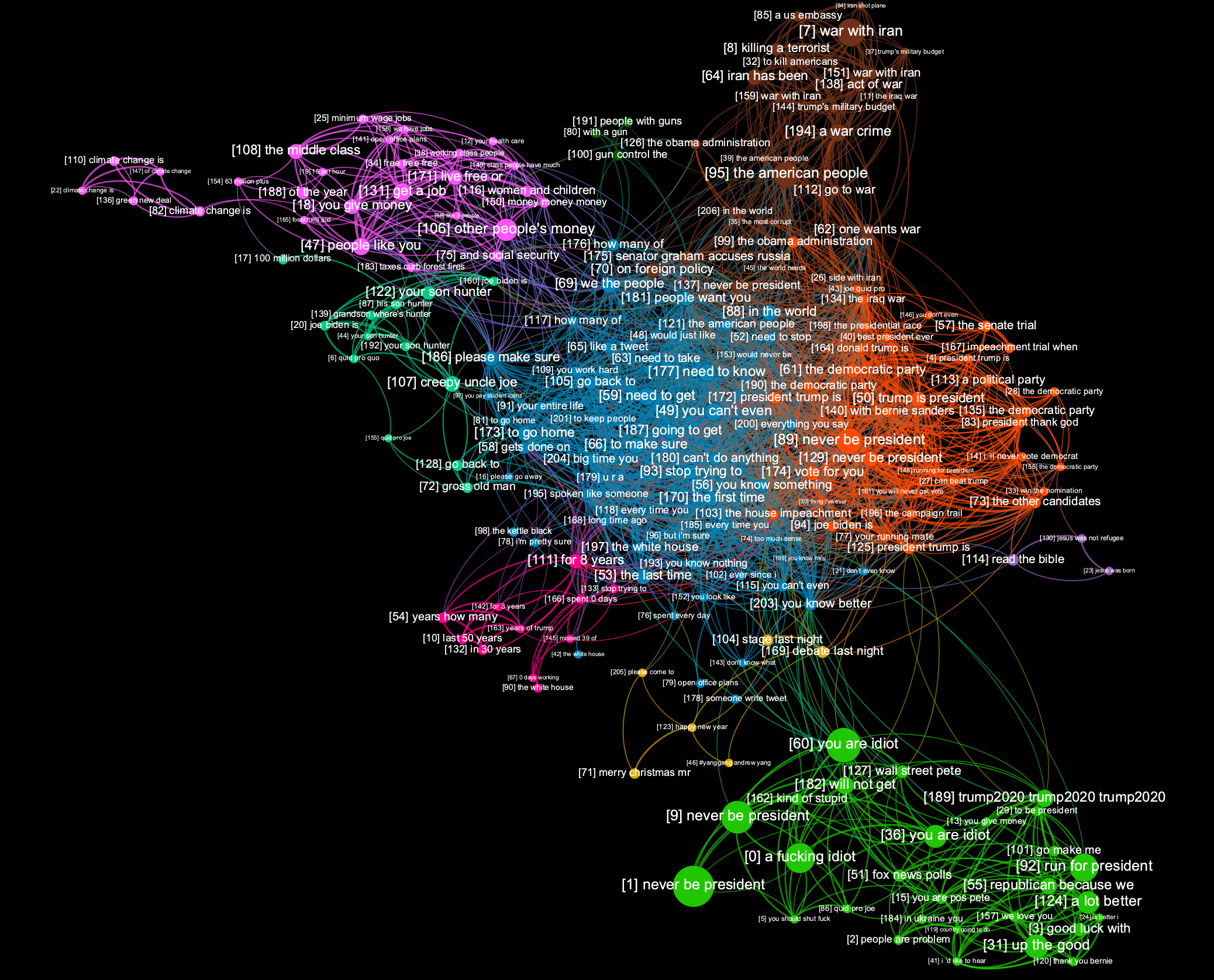
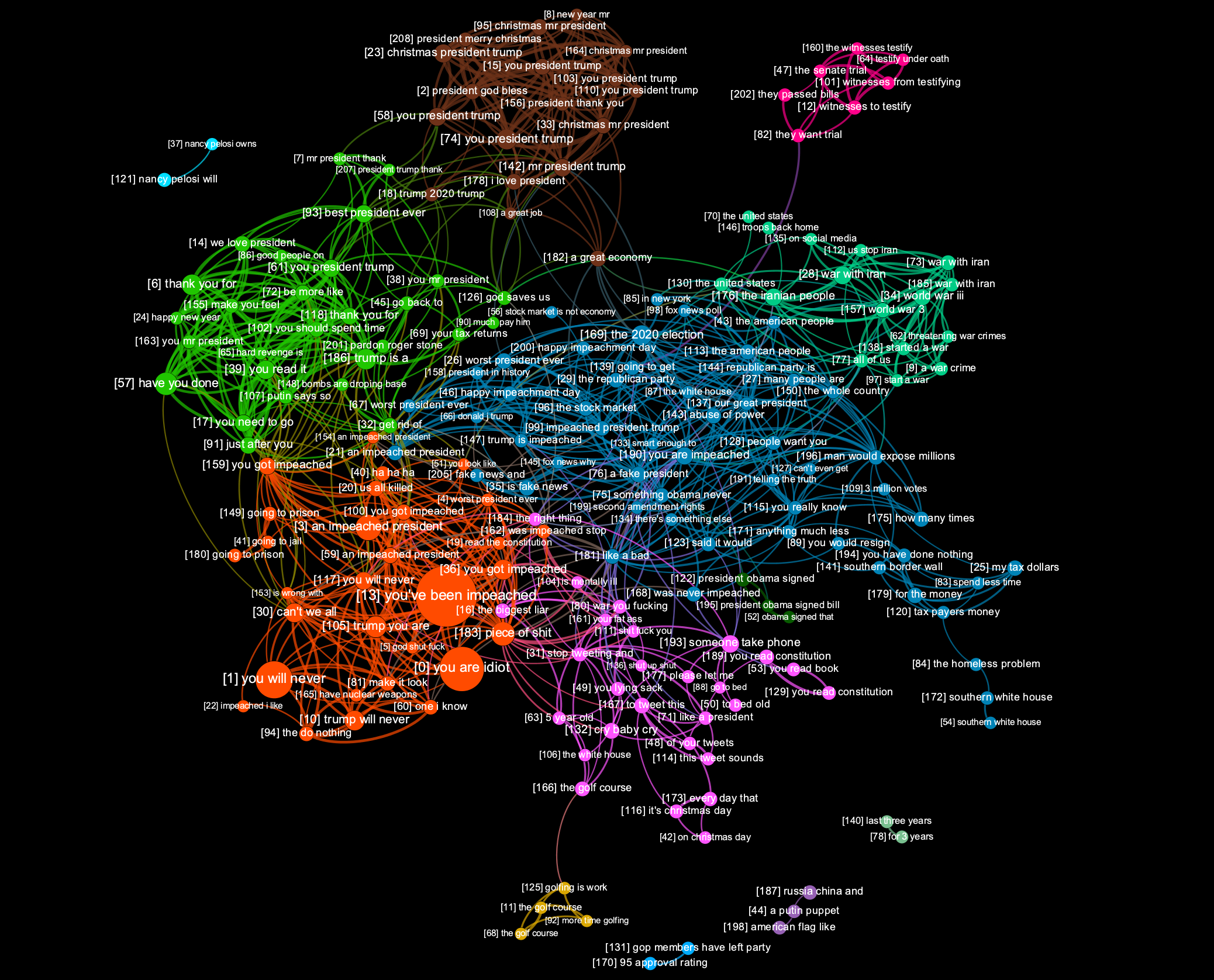
Our second experiment involved clustering of a subset of data in set 2 (@realDonaldTrump). We processed a batch of 30,044 tweets, resulting in 209 clusters.
A image below is a static graph visualization of the discovered clusters:
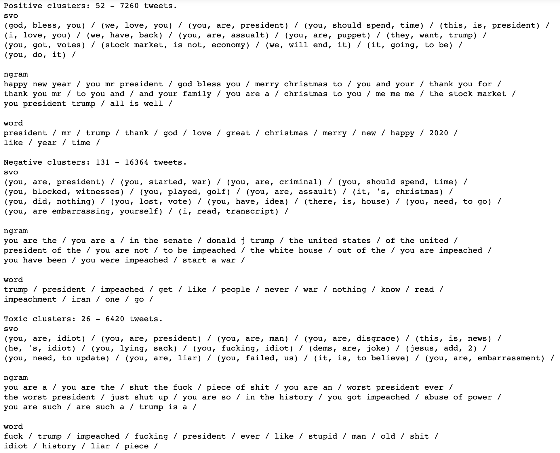
Using the same methodology as in our first experiment, we separated the clusters into positive, negative, and toxic, and then summarized them. Positive clusters included both statements of thanks and wishes of Merry Christmas and a Happy New Year, but also included the incorrectly categorized phrase “you are a puppet”. A summarization of negative clusters didn’t find any obvious false-positives, and included themes such as recent impeachment hearings, and comments on the amount of time the president has spent playing golf. Clusters deemed toxic contained, as expected, a lot of profanity.
Final values for this set were as follows:
Positive tweets: 7260 (24.16%) Negative tweets: 16364 (54.47%) Toxic tweets: 6420 (21.37%)
Note how @realDonaldTrump received a great deal more toxic replies than any of the accounts studied in the previous dataset. Note also that tweets contained in negative and toxic clusters totalled roughly three times that of tweets in positive clusters.
Here are some details from the largest identified clusters. They include the following negative themes:
-
You are an idiot/liar/disgrace/criminal/#impotus
-
You are not our president
-
You have no idea / you know nothing
-
You should just shut up
-
You can’t stop lying
-
References to Vladimir Putin
Here are some of the positive themes identified in these larger clusters:
-
God bless you, Mr. President
-
We love you
-
You are the best president
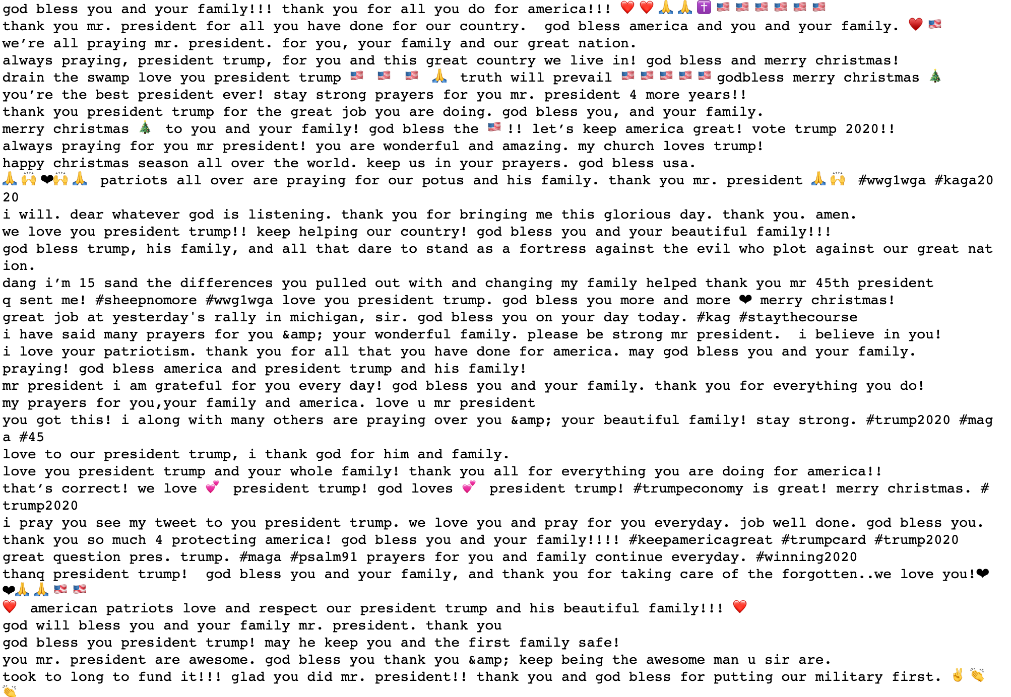
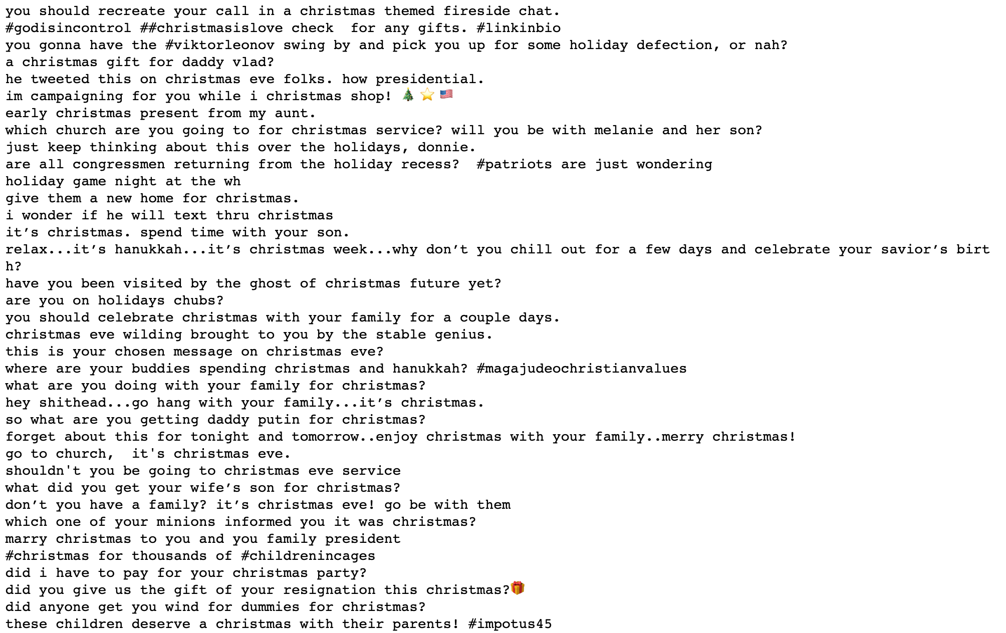
Above and below are Christmas-themed clusters, but with quite different messages. The one above contains mostly season’s greetings, whilst the one below contains some questions to Trump about his plans for the holidays.
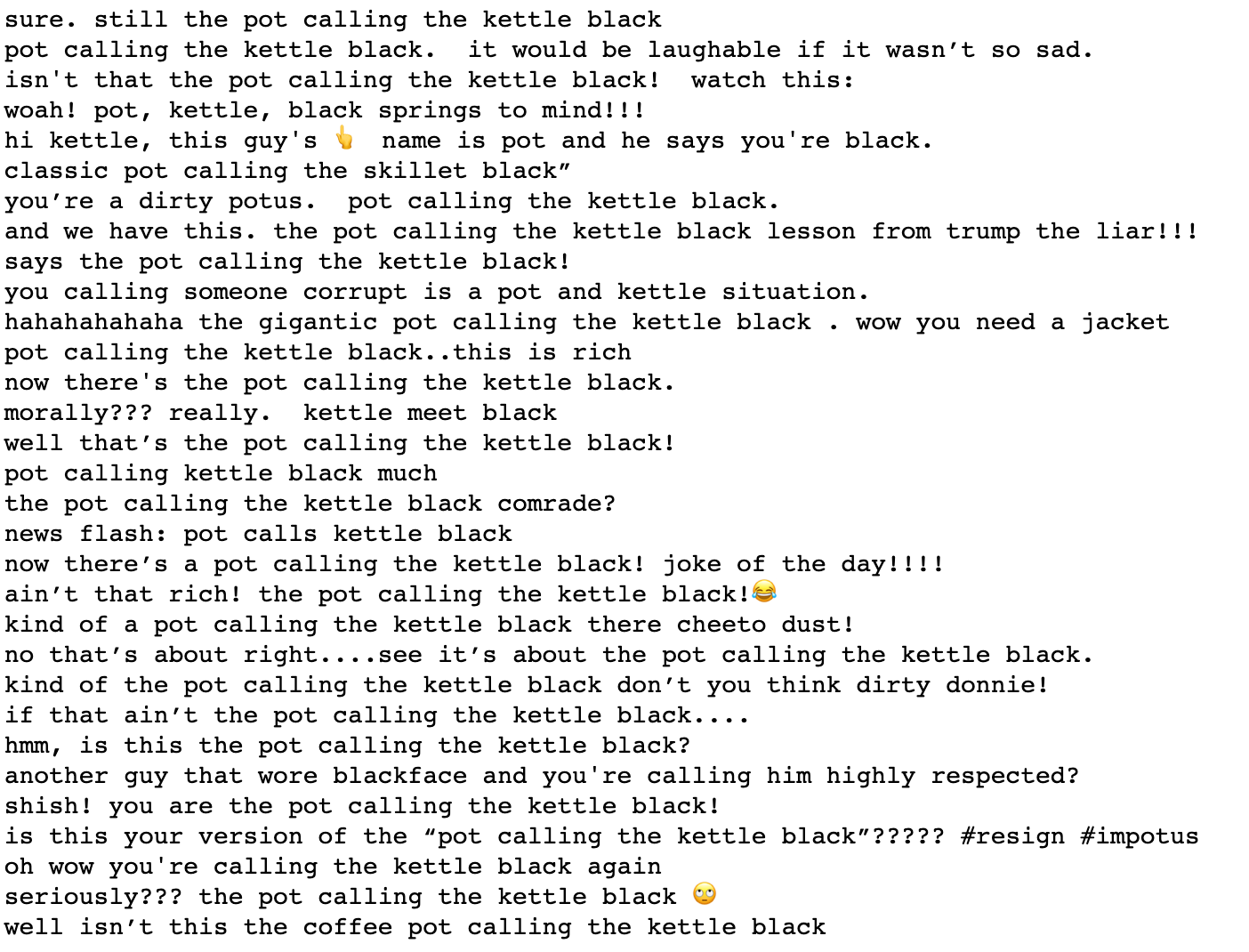
Below is a cluster that found a bunch of “pot calls the kettle black” phraseology. Note how it captures quite different phrases such as “name is pot and he says you’re black”, “kettle meet black”, “pot and kettle situation” and so on. It did fail on that one tweet that references blackface.
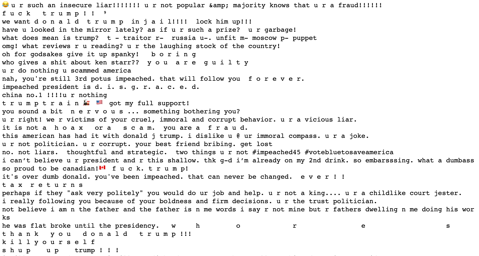
This next one (below) is interesting. It found tweets where people typed words or sentences with spaces between each letter.
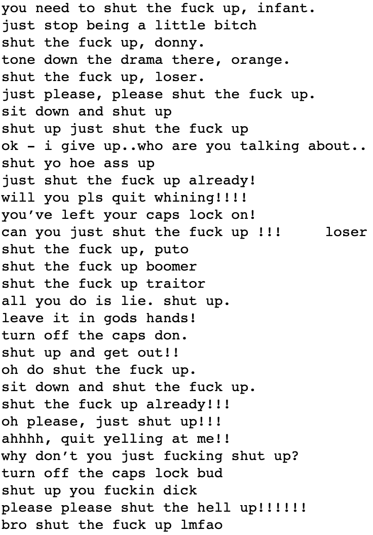
Below is a cluster that identified “stfu” phraseology.
Example output from this dataset (and others studies) can be found in our github repo (https://github.com/r0zetta/meta_embedding_clustering/tree/master/example_output).
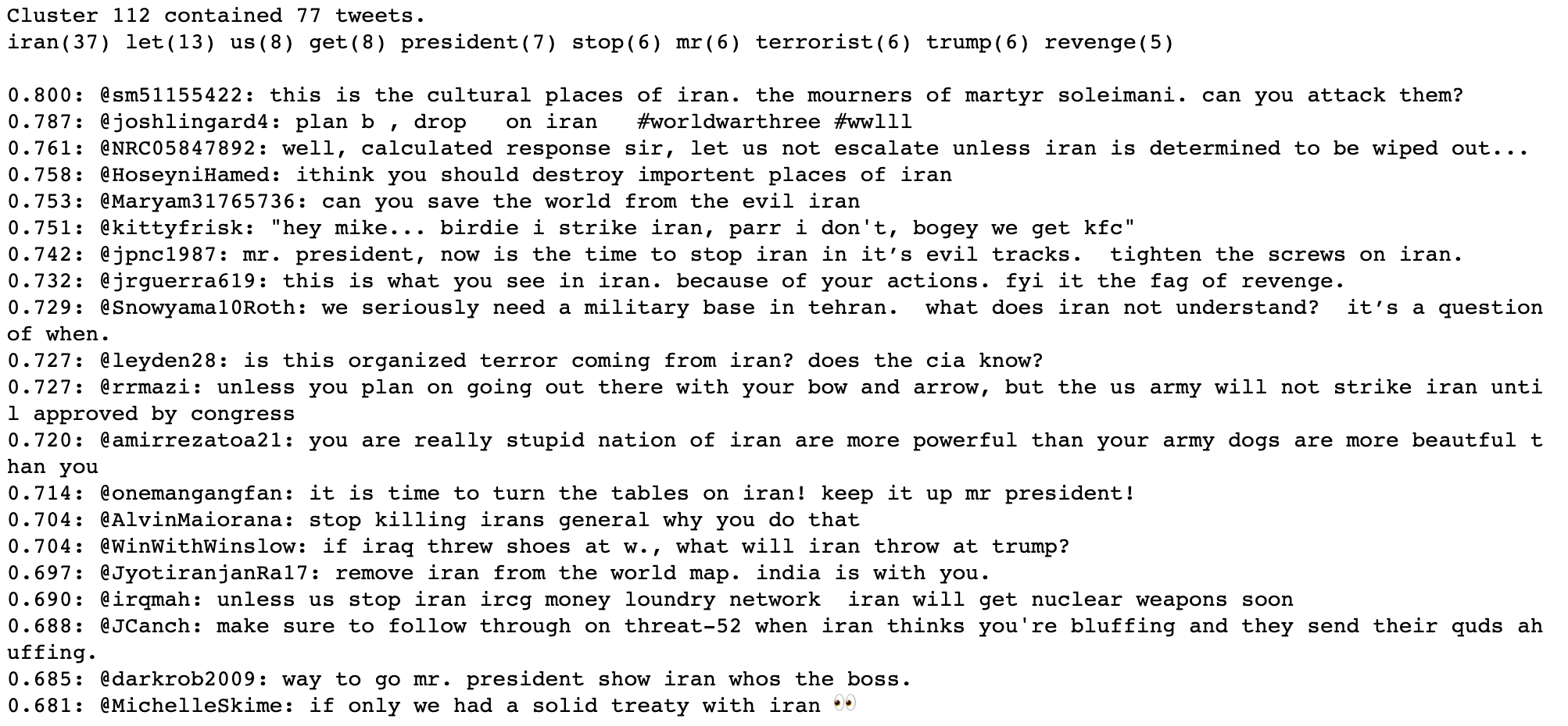
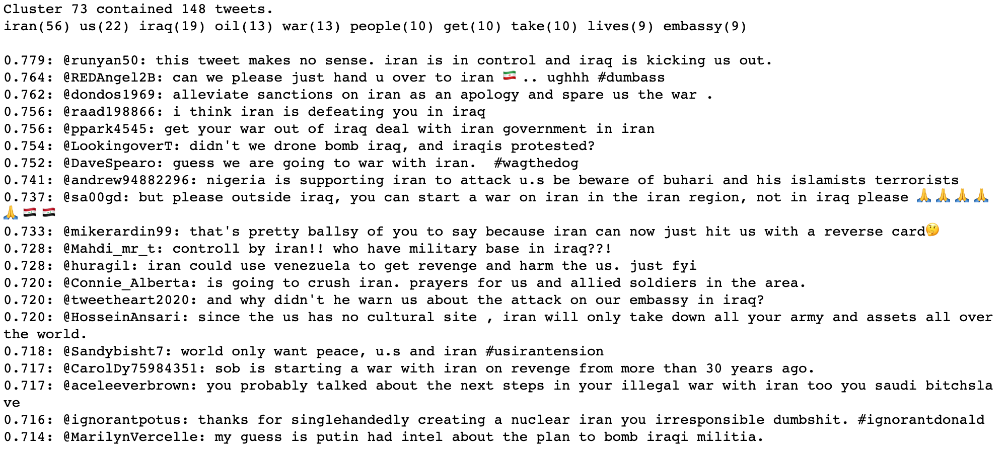
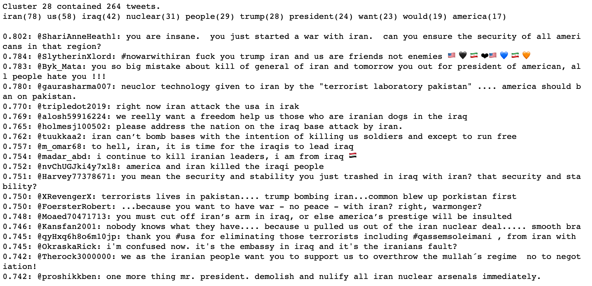
As mentioned in our methodology section (later in this article), the technique we’re using does sometimes identify multiple clusters containing similar subject matter. While looking through the clusters identified from replies to @realDonaldTrump, we found four clusters that all contained high percentages of tweets about a recent situation in Iran. Upon inspection we realized that those clusters contained different takes on the same issue.
Below is a cluster that contains some tweets praising Trump’s actions in the region.
Below is a cluster that contains some tweets mentioning Iraq and related repercussions of actions against Iran.
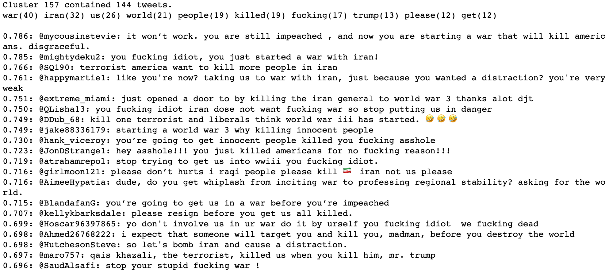
Below is a cluster that contains mostly negative comments about Trump’s actions in the region.
And finally, the cluster below contains a great deal of toxic comments.
We tested our topic modeling methodology further by running the same toolchain on a set of tweets collected during the run-up to the UK elections. These were tweets captured on hashtags relevant to those elections (#GE2019, #generalelection2019, etc.). Our methodology turns out to be quite well-suited for finding spam. Here are a few examples:
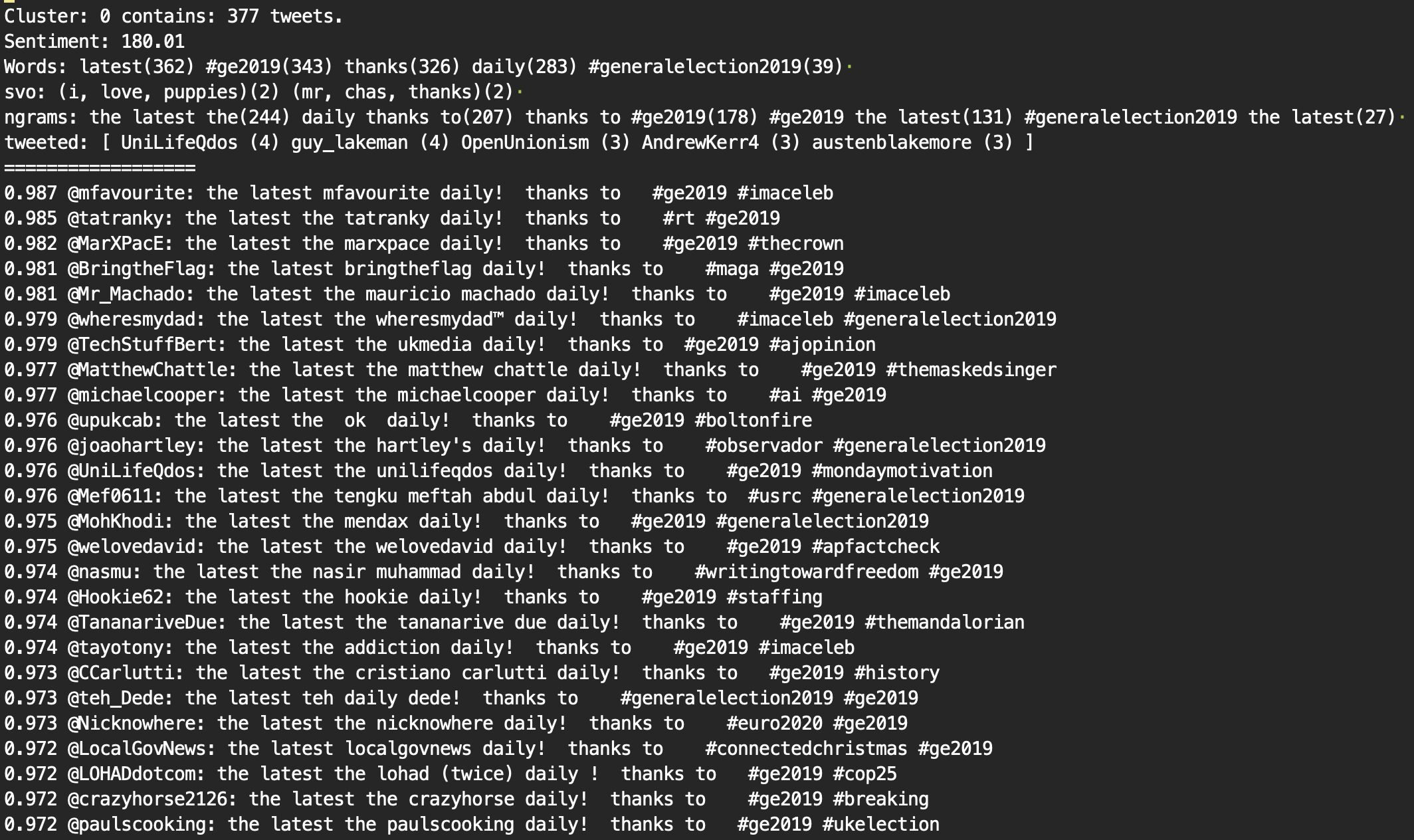
The output below contains tweets posted by an app called “paper.li”, which is a legitimate online service that folks can use to craft their own custom newspaper. It turns out there were a great deal of paper.li links shared on top of the #ge2019 hashtag. Unfortunately, this was one of four clusters identified that contained similar-looking paper.li tweets (which could be found more easily by filtering collected Twitter data by source field).
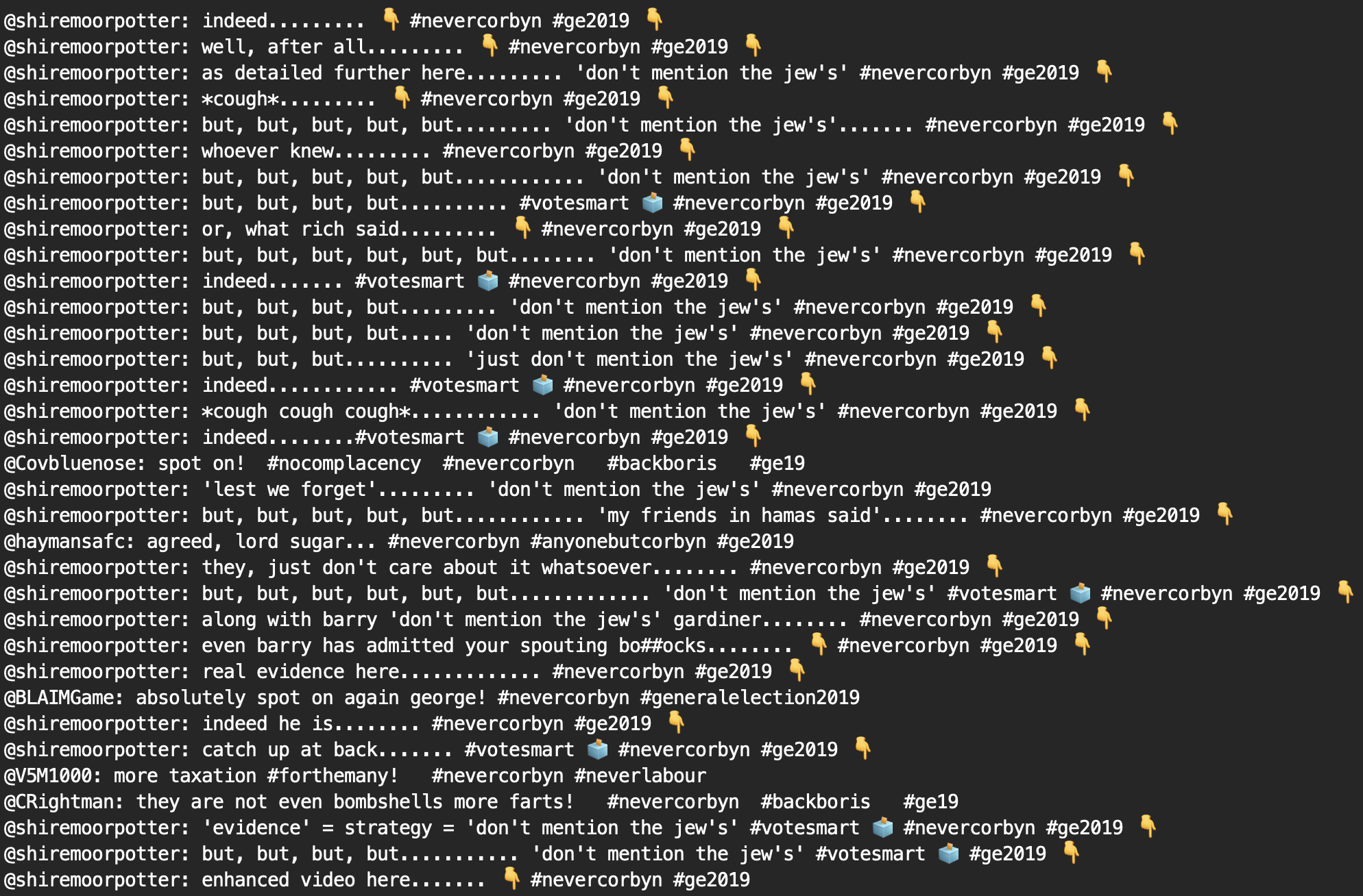
Below we can see some copy-paste disinformation, all shared by the same user. Note that this analysis was run over roughly 30,000 randomly selected tweets from a dataset with millions of entries. As such, I imagine we'd likely find more of the same from this user if we were to process a larger number of tweets.
Below we see some tweets advertising porn, on top of the #ge2019 hashtag. Spam advertisers often piggyback their tweets on trending hashtags, and the ones we captured trended often during the run-up to the 2019 UK general elections.
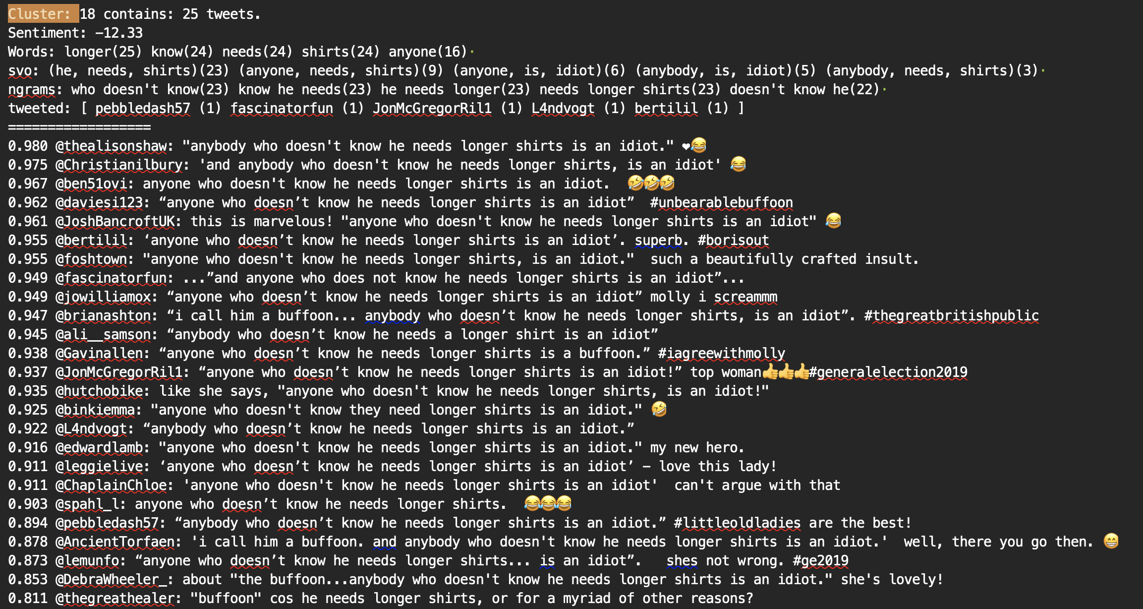
A cluster that identified a certain style of writing also identified tweets coming mostly from one account. Rather useful.
The cluster below picked up on similar phraseology. Not sure what that conversation was about.
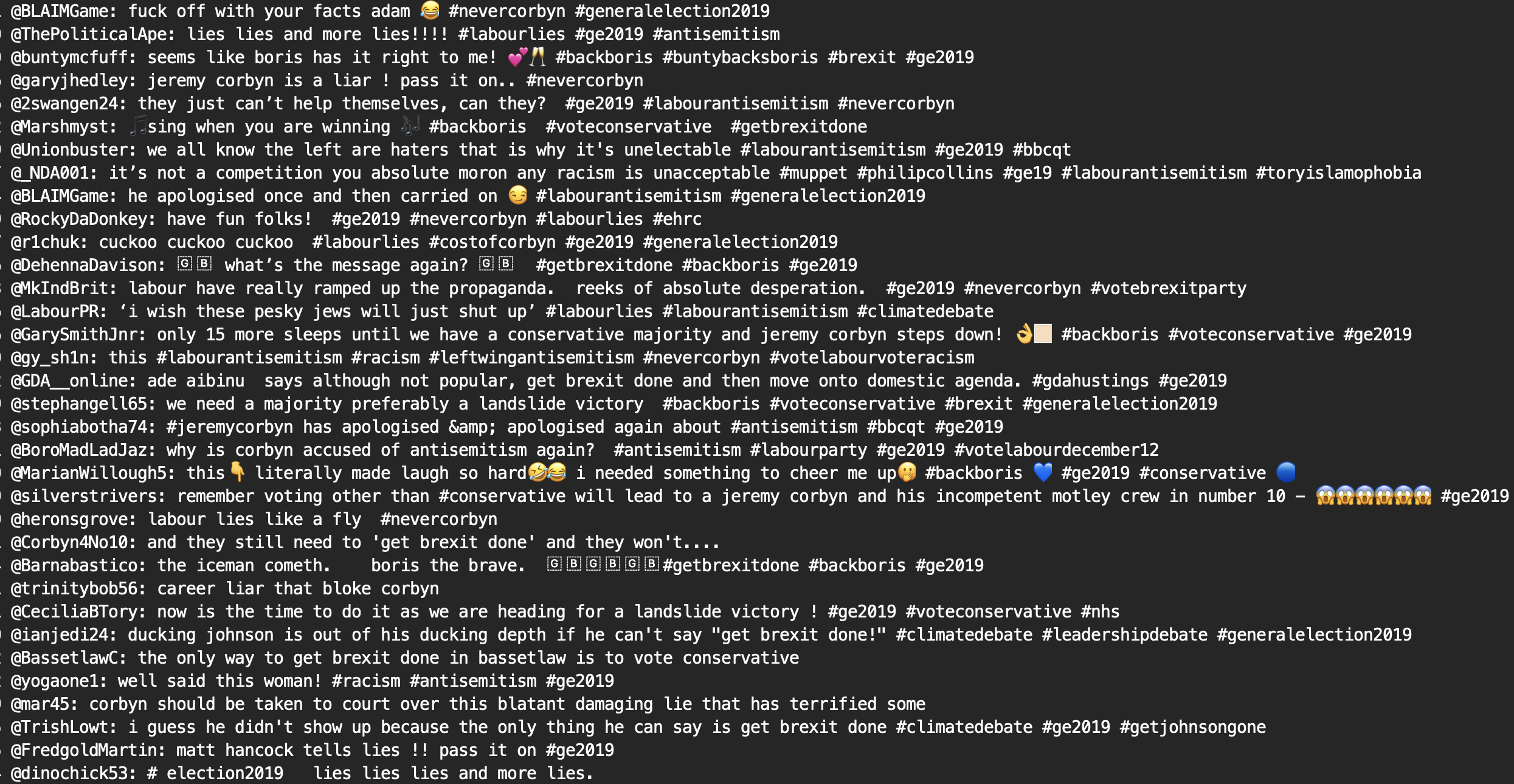
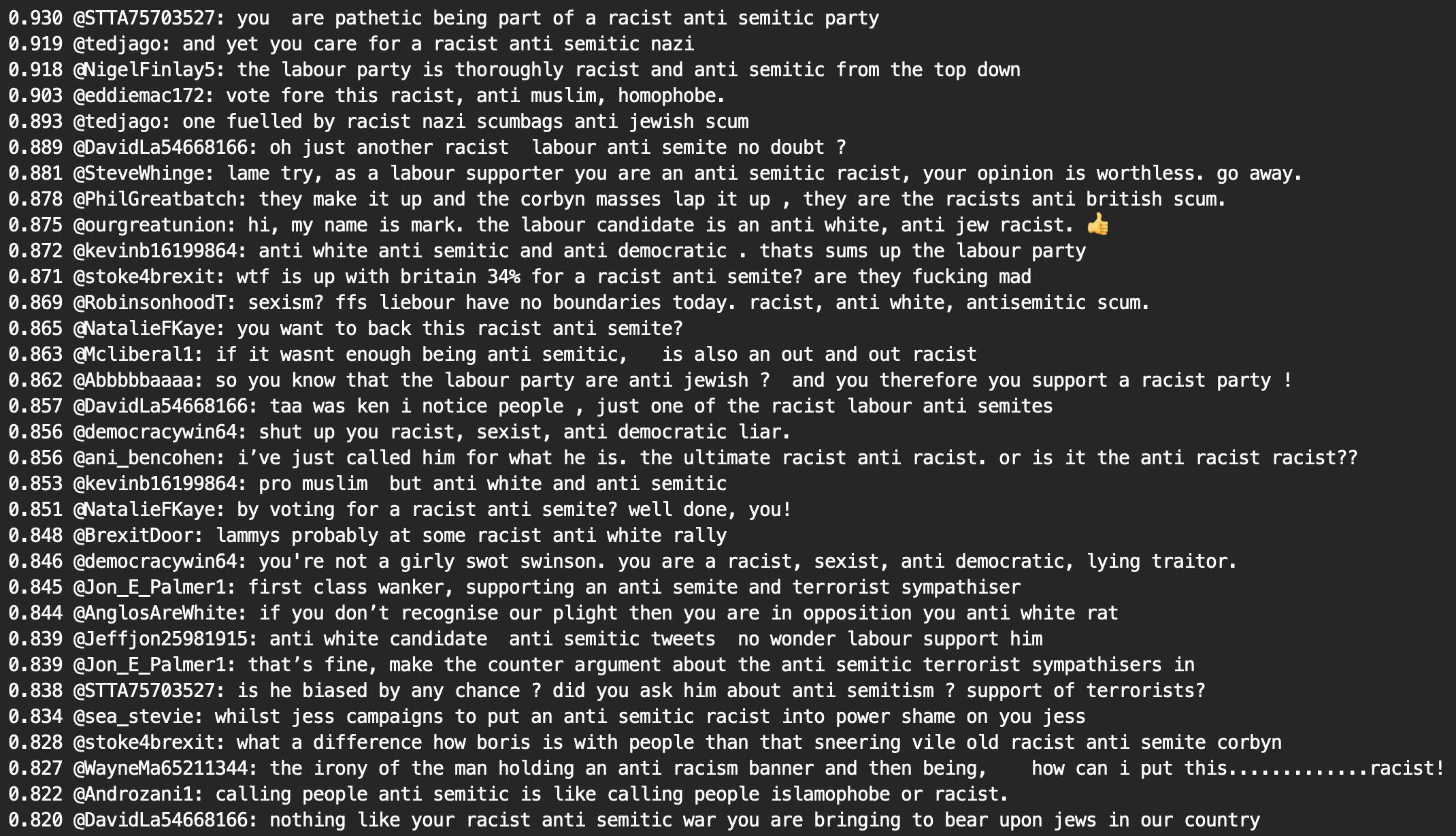
Finally, several clusters (shown below) contained a great deal of tweets including the word “antisemitism”. Many of the accounts in these clusters could be classified as trolls and/or fake disinformation accounts.
Note that we found similar clusters in data collected by following pro-tory activist accounts and sockpuppets during the same time period (shown below):
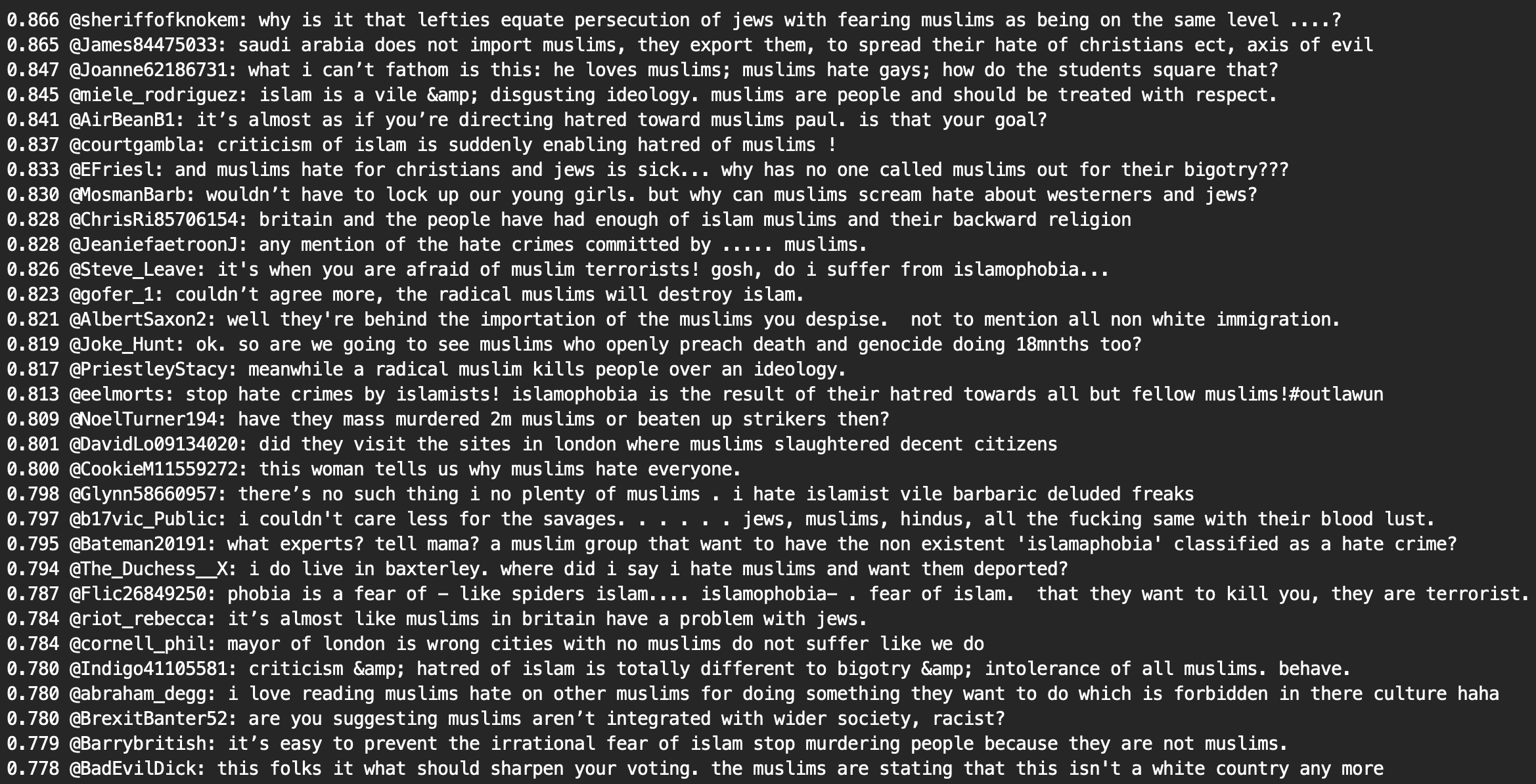
Other clusters were discovered in tweets from the same tory accounts, including a few that contained tweets designed to incite hatred towards specific demographics (see below)
It’s worth noting that a portion of the accounts identified in our clustered data have been suspended since the data was originally collected. This is a good indication that some of the users who post frequent replies to politicians, and participate in harassment are either fake, or are performing activities that break Twitter’s terms of service. Any methodology that allows such accounts to be identified quickly and accurately is of value.
The methodology developed for our experiments yielded a mechanism for grouping tweets with similar content into reasonably accurate clusters. It did a very efficient job at identifying similar tweets, such as those posted by coordinated disinformation groups, from reply-spammers, and from services that post content on behalf of a user’s account (such as paper.li or share buttons on web sites). However, it still suffers from a tradeoff between accuracy and the creation of redundant clusters. Further work is needed to refine the parameters and logic of this methodology such that it is able to assign groups of relatively rare tweets into small clusters, while at the same time creating large clusters of similar content, where appropriate.
In order to fully automate the detection of toxic content and online harassment, additional mechanisms must be researched and added to our toolchain. These include an automated method for creating rich, readable summaries of the contents of a cluster, more accurate sentiment or stance analysis of the contents of a cluster, and better methods for automatically assigning verdicts, labels, or categories to each cluster.
Further research into whether the identified clusters may be used to classify new content is another area worth exploring (initial experiments into this line of research are documented in appendix 2 of this article).
If these future goals can be completed successfully, a whole range of potential applications open up, such as, automated filtering or removal of toxic content, an automated method to assign quality scores to accounts based on how often they post toxic content or harass users, and the ability to track the propagation of toxic or trolling content on social networks (including, perhaps, behind-the-scenes identification of how such activity is coordinated).
This section contains a detail explanation of the methodology we employed to cluster tweets based on their textual content. Since this section is fairly dry and technical, we opted to leave it until the end of this article. Feel free to skip it unless you’re interested in replicating it for your own means, are involved in similar research, or are both curious and patient
All the code used to implement this can be found in our github repo (https://github.com/r0zetta/meta_embedding_clustering).
Twitter data was collected using a custom python script leveraging the Twarc module. The script utilized Twarc.filter(follow=accounts_to_follow) to follow a list of Twitter user_ids, and only collect tweets that were direct replies to accounts_to_follow list provided. Collected data was abbreviated (a subset of all status and user fields were selected) and appended to a file on disk. Once sufficient data had been gathered, the collection was terminated, and subsequent analyses were performed on the collected data.
Collected Twitter data was read from disk and preprocessed in order to form a dataset of relevant tweets. Tweet texts were stripped of urls, @mentions, leading, and trailing whitespace, and then tokenized. If the tweet contained enough tokens, it was recorded, along with information about the account that published the tweet, the account that was replied to, and the tweet's status ID (in order to be able to recreate the original URL). Both the preprocessed tweet texts and tokens were saved during this process.
Three different sentence vectors were then calculated from each saved tweet:
-
A word2vec model was trained on the tokenized tweets. Sentence vectors for each tweet were then calculated by summing the vector representations of each token in the tweet.
-
A doc2vec model was trained on the preprocessed tweet texts. Sentence vectors were then evaluated for each preprocessed tweet text.
-
BERT sentence vectors were calculated for each preprocessed tweet text using the model's encode function. Note that this can be a rather time-consuming process.
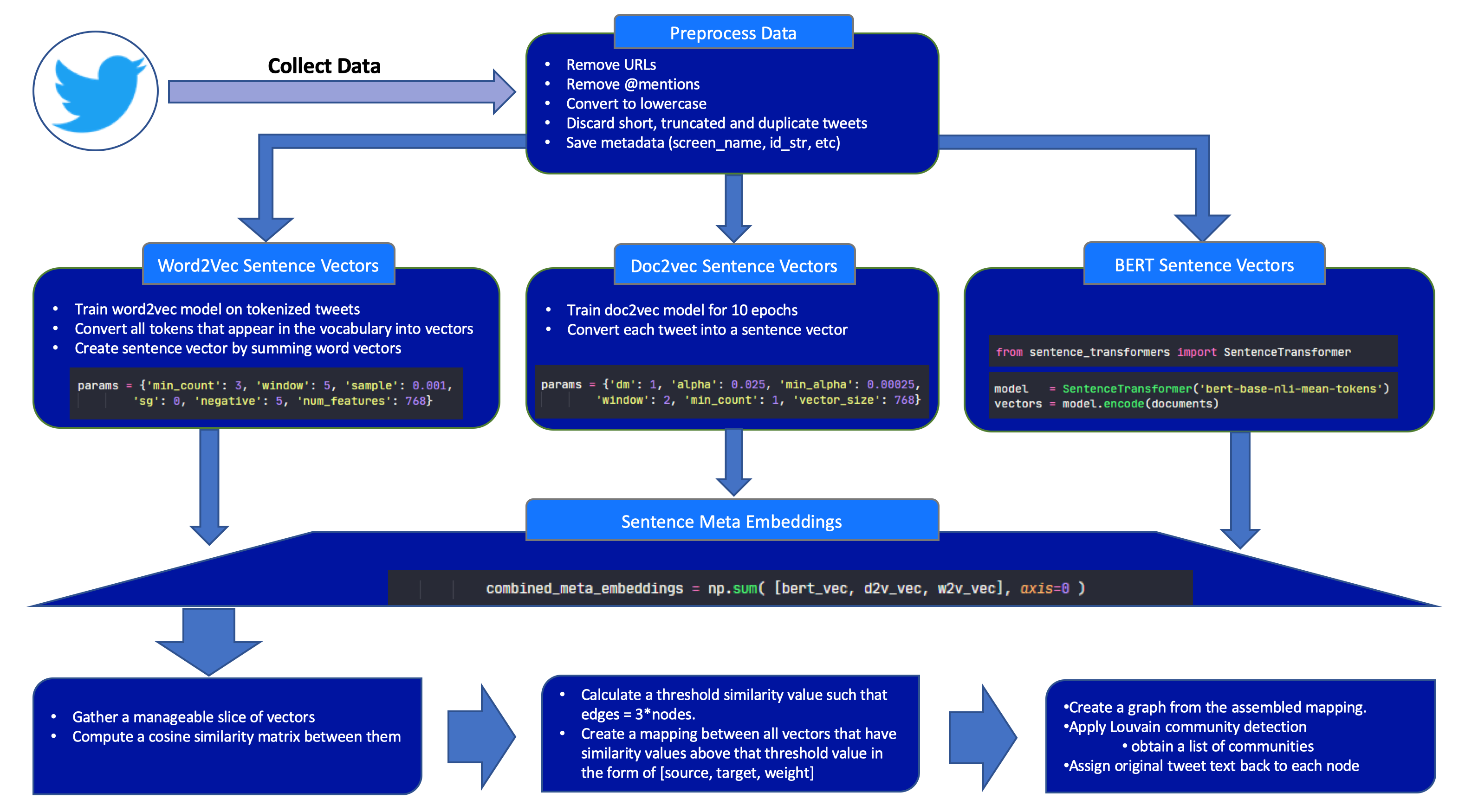
Sentence meta embeddings were then calculated by summing the three sentence vectors calculated for each tweet. The resulting sentence meta embeddings were then saved in preparation for the next step.
Traditional methods for clustering textual data (such as Latent Dirichlet Allocation) require text to be stemmed and/or lemmatized (the process of reducing inflected words to their word stem, base, or root form). This process can be cumbersome and inaccurate. Since embeddings capture relationships between similar words in an unsupervised manner, our approach does not require either stemming or lemmatization.
Our clustering methodology involves the following steps:
-
Calculate a cosine similarity matrix between vector representations of the sentences meta embeddings for a batch of samples. This process generates a matrix of similarity values between all possible pairs of vectors in the sample batch.
-
Calculate (or manually set) a threshold value at which we would draw an edge between two nodes in a graph.
-
Find all vector pairs that have a cosine similarity equal to or greater than the threshold value. Create a node-edge graph from these values, setting the edge weight equal to the cosine similarity between that pair of vectors.
-
Perform Louvain community detection on the resulting graph. This process labels each node based on the community it was assigned to.
-
Process the results of the clustering - for instance, extract common words, n-grams, and subject-object-verb triplets.
-
Perform manual inspection and statistical analysis of the resulting output.
Here is a diagram of the above process:
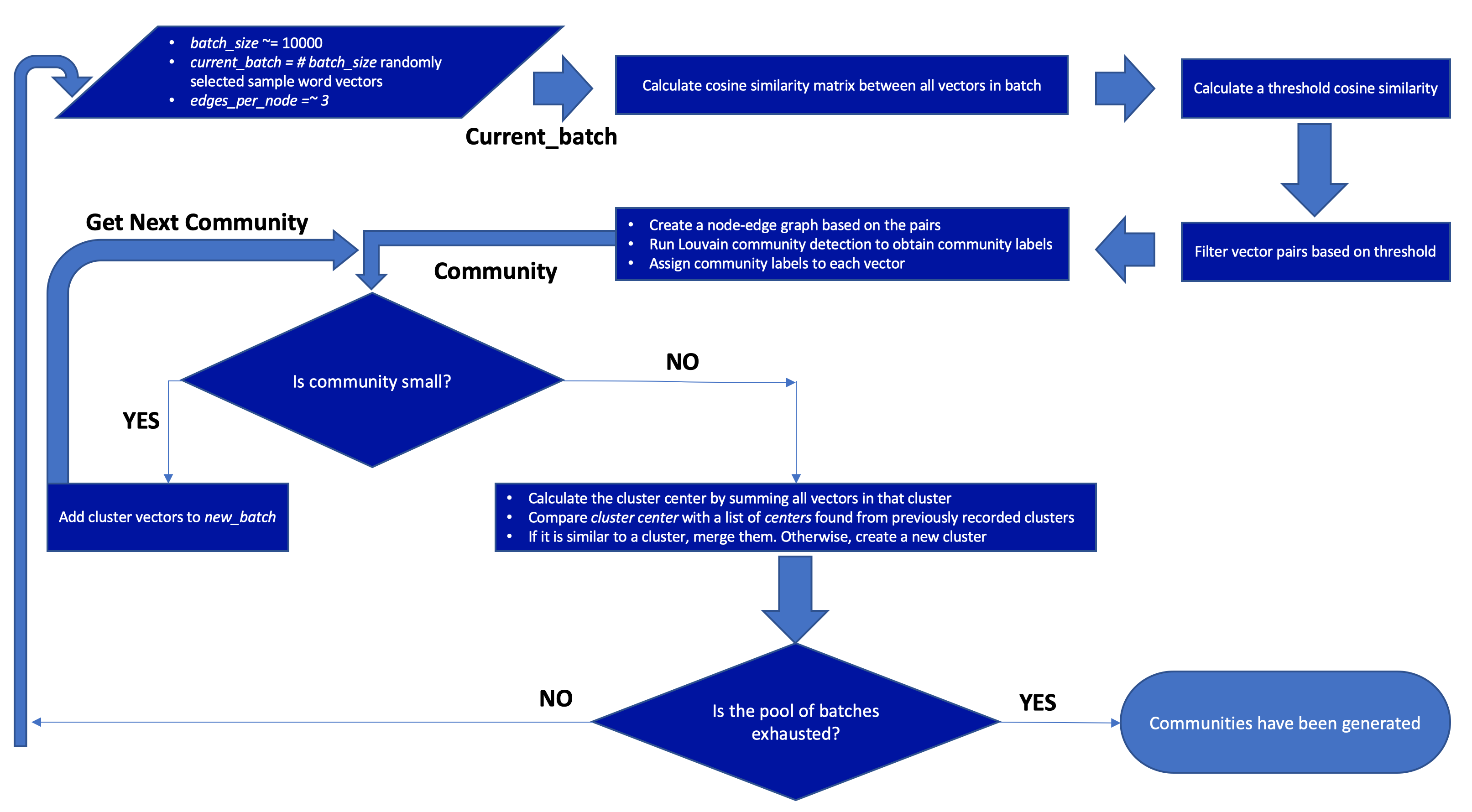
It is possible to perform reasonably fast (less than 10 seconds) in-memory cosine similarity matrix calculations on small sets (<20000) using, for instance, the sklearn.metrics.pairwise cosine_similarity function. However, larger sets of vectors that don't fit into memory require a calculation loop that can take anywhere between minutes and hours to run. In order to process our large sample sets, we opted to perform processing in batches using the following logic:
-
Start with an array, current_batch, populated with small batch_size (e.g. 10,000) randomly selected sample vectors from the full set of samples to be clustered. We used randomly sampled vectors during all of our experiments so as to not optimize clustering logic for a deterministic set of inputs.
-
Calculate an in-memory cosine similarity matrix between all vectors in current_batch.
-
Calculate a threshold cosine similarity value that will select the top (batch_size * edges_per_node) samples from current_batch.
-
Iterate through the cosine similarity matrix values found for vectors in current_batch, adding pairs of nodes to a list, graph_mapping, in the form [source, target, cosine_similarity] for each pair whose cosine similarity was equal to or greater than the threshold value calculated in the previous step.
-
Create a node-edge graph using the graph_mapping list created in the previous step. Edge weights are assigned to the cosine_similarity values obtained during that process. Run the Louvain community detection algorithm on the graph to obtain a list of nodes, labeled by community. This process will not utilize all of the vectors in current_batch, so save a list of vectors that were not included in the resulting graph into a new list, new_batch.
-
Iterate through the communities found in the previous step, selecting the list of vectors that were assigned to each community.
-
If the length of the list of vectors assigned to a community is less than the defined minimum_cluster_size, add those vectors to new_batch and proceed to the next community.
-
If the length of the list of vectors assigned to a community is equal to or greater than the defined minimum_cluster_size, continue processing that cluster.
-
For each cluster that fits the minimum_cluster_size requirement, calculate a cluster_center vector by summing all vectors in that cluster. Compare cluster_center with a list of cluster_center values found from previously recorded clusters. If the new cluster center has a cosine similarity value that exceeds a merge_similarity value, assign items to the previously recorded cluster. If not, create a new cluster, and assign items to that.
-
Once all communities discovered in step 5 have been processed, add new samples from the pool to be processed to new_batch until it reaches size batch_size, assign it to current_batch, and return to step 1. Once all samples from the pool have been exhausted, or the desired number of samples have been clustered, exit the loop.
Here is a diagram of the above process:
Occasionally, the loop runs without finding any communities that fulfill the minimim_cluster_size requirement. This, of course, causes the loop to go infinite. We added logic to detect this (check that the length of new_batch is not the same as batch_size before proceeding to the next pass). Our fix was to forcefully remove the first 10% of the array and append that many new samples to the end before proceeding to the next pass.
Different batch sizes result in quite different outcomes. If batch_size is small, the selection of samples used to create each graph may not contain a wide enough variety of samples from the full set, and hence samples will be missed. If batch_size is large, more communities are discovered (and the calculations take longer, require more memory, etc.). We found that setting batch_size to 10,000 was optimal in terms of accuracy, speed, and memory efficiency.
The edges_per_node variable has a marked effect on the accuracy of the clustering process. When edges_per_node is set to a low value (1-3), less samples are selected from each batch during graph creation, and community detection often finds many very small (e.g. 2-item) communities. However, when edges_per_node is set to higher values (>6), a smaller number of larger communities are detected. However, these communities can contain multiple topics (and hence are inaccurate). We found that an edges_per_node value of 3 to be optimal for a batch_size of 10,000. Increasing batch_size often requires also increasing edges_per_node to achieve similar looking results.
The minimum_cluster_size variable affects the granularity of the final clustering output. If minimum_cluster_size is set to a low value, more clusters will be identified, but multiple, redundant clusters may be created (that all contain tweets with similar subject matter). If accuracy is not important, setting minimum_cluster_size to a higher value will result in less clusters, and less redundancy, but may create clusters containing multiple topics (false positives), and may cause some topics to be lost. In datasets that contain a very wide range of different topics, a high minimum_cluster_size value (e.g. 50) may cause the process to not find any relevant communities at all. We found this variable to be very dataset-dependent. We tried values between 5 and 50, but ended up using a value of 50 for our experiments, mostly to allow for aesthetically pleasing visualizations to be created.
The merge_similarity variable has a similar effect on the output as the edges_per_node variable discussed earlier. This variable dictates the threshold at which newly identified clusters are merged with previously discovered ones. At lower values, this variable may cause multiple different topics to be merged into the same cluster. At high values, more redundant topic clusters are created. In our setup, we set merge_similarity to 0.98.
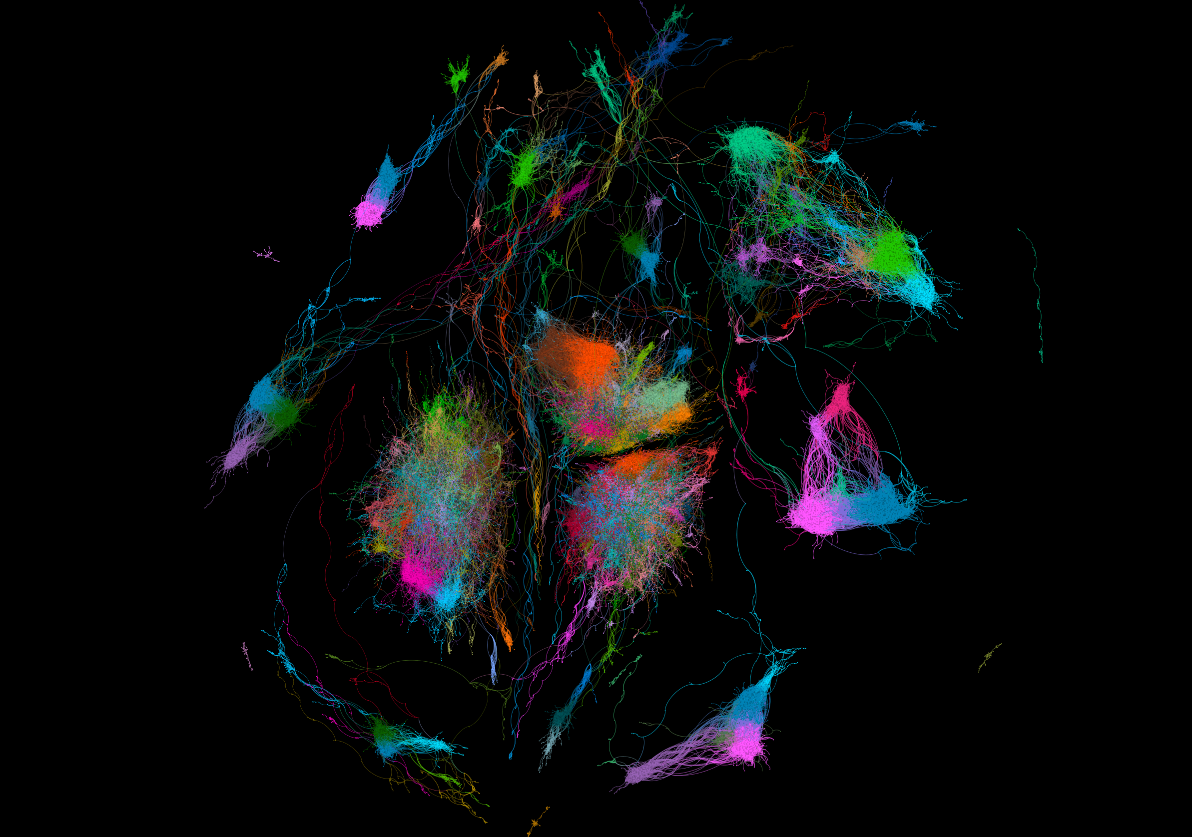
An example of a visualized graph (the one we generated using 30k tweets from set 1) looks like this:
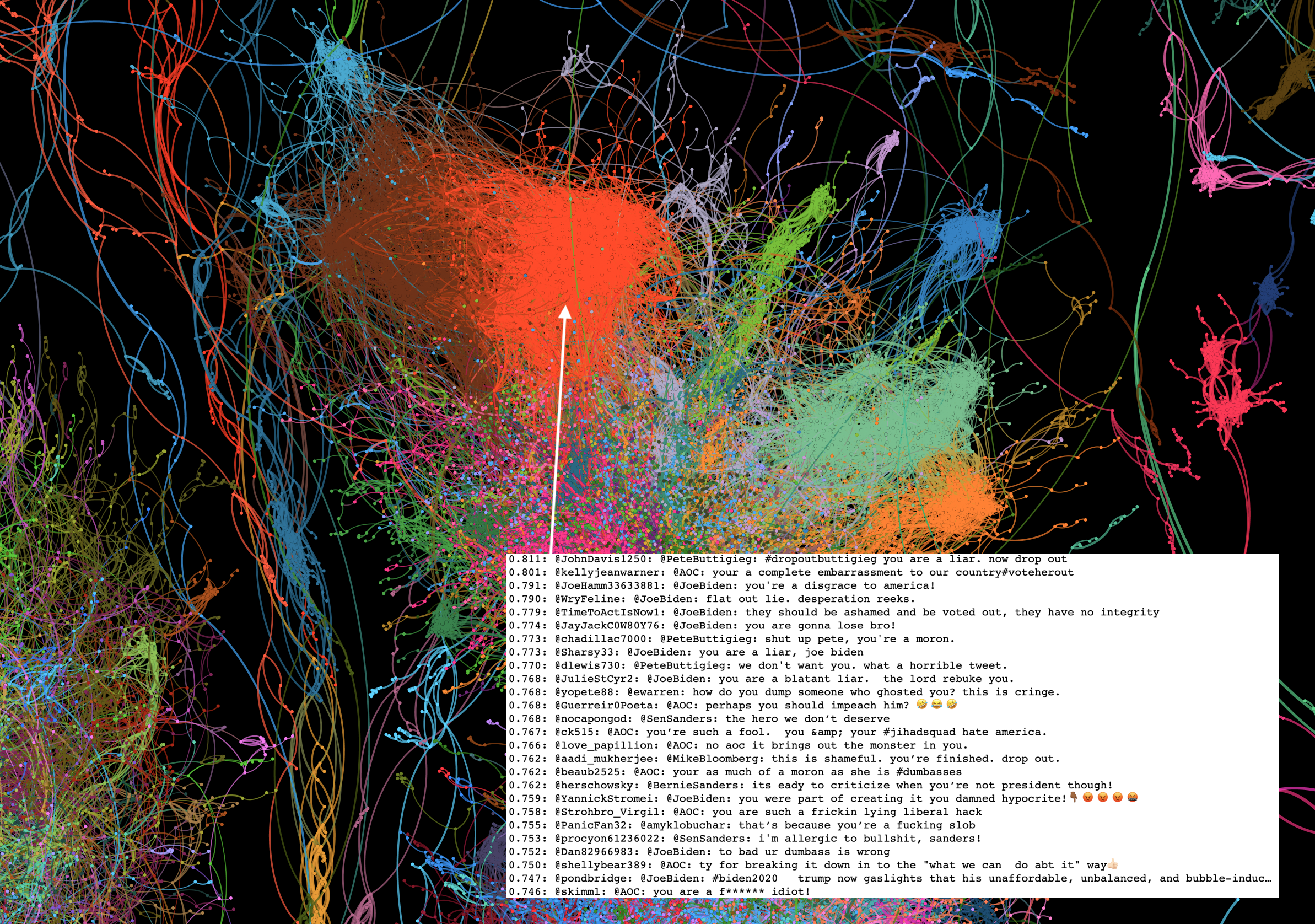
Below are a few examples of how tweets assigned to identified clusters map onto the visualized graph:
We experimented with the idea that identified clusters might be used to classify new tweets. In order to do this, we clustered approximately 25% of all tweets from each dataset and then attempted to classify the entire captured dataset using the following process:
1. For each tweet in the dataset, calculate meta embeddings using the same models and methods that were used to generate the clusters.
2. Run cosine similarity between the new tweet's meta embedding and all previously identified cluster centers, and find the best match (highest cosine similarity score).
3. If the cosine similarity exceeds a threshold, label that tweet accordingly. If not, discard it. In this case, we used a value of 0.65 as a threshold.
Set 1 (democrats):
184,851 (approximately 25% of the full dataset) tweets were clustered (using a minimum_cluster_size of 5) to obtain 3,376 clusters. The full 719,617 set of tweets were then converted into sentence meta embeddings and compared to the clusters found. This process matched 541,812 (75.29%) of the tweets.
Set 2 (realDonaldTrump):
188,010 (approximately 25% of the full dataset) tweets were clustered (using a minimum_cluster_size of 5) to obtain 3,894 clusters. The full 747,232 set of tweets were then converted into sentence meta embeddings and compared to the clusters found. This process matched 623,120 (83.39%) of the tweets.
By manually inspecting the resulting output (lists of tweet texts, grouped by cluster) we were able to determine that while some newly classified tweets matched the original cluster topics fairly well, others didn't. As such, identified cluster centers can’t reliably be used as a classifier to label new tweets from data captured with similar parameters. When using a threshold value higher than 0.65, a lot less tweets ended up being matched to existing clusters. One possible reason for the failure of this experiment is that some identified clusters contain tweets that only have very high cosine similarity values to the cluster center (above 0.95), whilst others contain tweets with much lower similarities (albeit whilst the content of the tweets match each other). As such, it might be that each cluster must have its own specific threshold value in order to match similar content. We didn't spend a great deal of time exploring this topic, but feel it may be worth researching in the future. Naturally, if this were figured out, cluster centers would likely only be valid for a short duration after they've been created due to the fact that the political and news landscape changes rapidly, and no techniques exist (as of yet) in this area that are able to create models that include a temporal context.
