knnstdisagg

An R package to perform space and time disaggregation of streamflow using a K-nearest neighbor (knn) approach.

Installation

Currently only available on GitHub

# install.packages("remotes")
remotes::install_github("rabutler-usbr/knnstdisagg")

Example Usage

One application of the KNN space-time disaggregation methodology is to take paleo reconstructed data at Lees Ferry in the Colorado River Basin, and disaggregate those annual flows at one location to monthly flows at 29 locations. The following steps through how to use the knnstdisagg package to do so.

As the space-time disaggregation method relies on monthly pattern data, we need monthly pattern data, and we will use the CoRiverNF package for those data.

remotes::install_github("BoulderCodeHub/CoRiverNF")

Setup the data

The space-time disaggregation disaggregates an annual value (ann_flow) to monthly data by matching ann_flow to an annual index value (ann_index_flow). Then, the monthly pattern and spatial pattern (mon_flow) from the selected annual index year is used to disaggregate the data.

In this example, we will be disaggregating the Meko et al. (2007) paleo reconstructed data (meko), which is provided as an example dataset in this package:

library(knnstdisagg)
library(CoRiverNF)
#> Loading required package: xts
#> Loading required package: zoo
#> 
#> Attaching package: 'zoo'
#> The following objects are masked from 'package:base':
#> 
#>     as.Date, as.Date.numeric
#> CoRiverNF package currently includes 1906-2018 natural flows, released January 10, 2020.

head(meko)
#>      water_year lees_ferry
#> [1,]        762   16360000
#> [2,]        763   13190000
#> [3,]        764   12140000
#> [4,]        765   12690000
#> [5,]        766   16660000
#> [6,]        767   14380000

meko is already formatted correctly for use in this package: one column of years and one column of annual data.

The annual index flow and monthly values are from the CoRiverNF package. We will match the meko data to the historical water year data at Lees Ferry. Additionally, for now, the index data needs to be a two column matrix and not an xts object. For the monthly data, we need it to be full water years, so need to remove the last three months of data so it stops at the end of the last water year.

# setup annual data
annual_index <- CoRiverNF::wyAnnTot$LeesFerry
yrs <- as.numeric(format(index(wyAnnTot$LeesFerry), "%Y"))
annual_index <- as.matrix(annual_index)
annual_index <- cbind(yrs, annual_index)

# setup monthly data
last_month <- paste0("/", max(yrs), "-09")
monthly_data <- CoRiverNF::monthlyInt[last_month]

Note, this example uses a named xts object for the monthly data, which means the results are also a named xts object. An unnamed matrix will also work.

Space-time disaggregation

The space-time disaggregation is performed by knn_space_time_disagg(). We have already setup the data necesary for ann_flow, ann_index_flow, and mon_flow. Because this is water year data, we will set the start_month to 10 as the water year starts in October. We will only disaggregate the data once, so there is only one “simulation”. In previous work, we have found that we want to scale the Upper Basin nodes based on the volume at Lees Ferry, but in the Lower Basin, we will not scale their values, i.e., we will select the monthly data directly for the selected index year. The Upper Basin sites are sites 1-20. Finally, we will use the default weighting scheme from Nowak et al. to select the nearest neighbor.

disagg <- knn_space_time_disagg(
  ann_flow = meko,
  ann_index_flow = annual_index,
  mon_flow = monthly_data,
  start_month = 10,
  nsim = 1,
  scale_sites = 1:20,
  k_weights = knn_params_default(nrow(annual_index))
)
#> Sites 21, 22, 23, 24, 25, 26, 27, 28, 29
#> will be selected directly from the index years, i.e., not scaled.

The results are now in disagg, and we can get the output using knnst_get_disagg_data():

head(knnst_get_disagg_data(disagg)[,5:10]) # only look at a few sites
#>         Crystal GrandJunction CiscoDolores CiscoColorado Fontenelle
#> 761-10 5034.272      84700.62    39670.062      6224.374   65747.59
#> 761-11 4631.530      36982.77    19135.267     14840.026   45308.45
#> 761-12 1610.967      34120.28     9108.005     10993.843   39267.32
#> 762-01 2114.394      27275.68     8234.055      3563.258   37253.61
#> 762-02 2617.821      34888.51    11017.000      5985.749   32219.34
#> 762-03 4832.901      33166.79    32489.177      9785.618   61418.12
#>        GreenRiverWY
#> 761-10    12585.680
#> 761-11     9263.060
#> 761-12     4027.417
#> 762-01     2919.878
#> 762-02     4128.103
#> 762-03    21445.998

If needed, the output can be saved to disk using write_knnst(). This saves the disaggregated data for every simulation as well as the selected index years.

QA/QC

Base Statistics

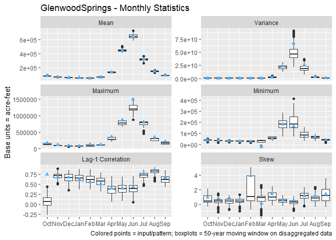
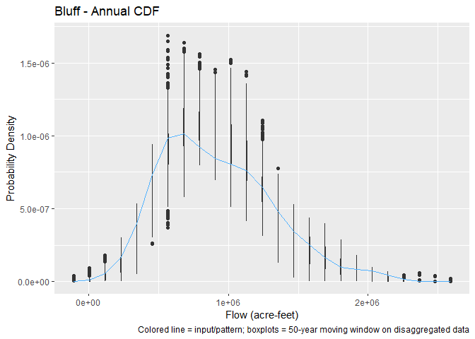
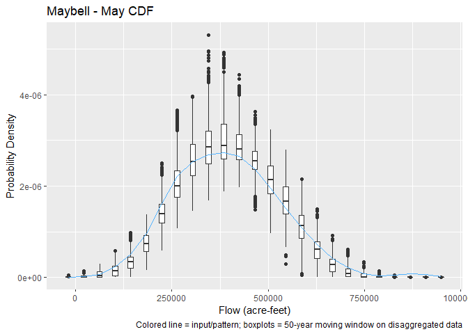
The knnstdisagg package also includes plotting functionality to assist with QA/QC. Plots of monthly statistics (mean, max, min, variance, lag-1 correlation, and skew), annual statistics (same as monthly), annual cdf, and a monthly cdf for each month can be created using plot(). Each call to plot works for one site. A bin_size must be specified; this is the moving window that all statistics on the disaggregated data are computed accross. Looking at Glenwood Springs monthly statistics:

p <- plot(
  disagg, 
  site = "GlenwoodSprings", 
  base_units = "acre-feet", 
  which = 14, 
  show = TRUE,
  bin_size = 50
)

If an unnamed matrix was used for input, then the sites are accessed by "S1", "S2", etc. during plotting.

We can also look at the annual cdf for Bluff, or the May cdf for Maybell:

p <- plot(
  disagg, 
  site = "Bluff", 
  base_units = "acre-feet", 
  which = 13, 
  show = TRUE,
  bin_size = 50
)

p <- plot(
  disagg, 
  site = "Maybell", 
  base_units = "acre-feet", 
  which = 5, 
  show = TRUE,
  bin_size = 50
)

All plots for a given site can be created at once using which = 1:15, and the suite of plots can be saved using save_knnstplot(). For example, all plots for the data at Cameo could be saved to a pdf using:

p <- plot(
  disagg, 
  site = "Cameo", 
  base_units = "acre-feet", 
  which = 1:15, 
  show = FALSE,
  bin_size = 50
)
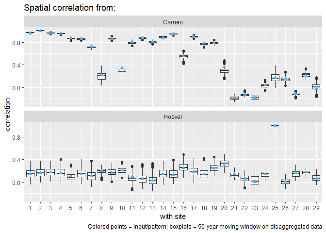
save_knnstplot(p, "Cameo.pdf", width = 8, height = 6)

Spatial Correlation

Another statistic to check is the spatial correlation between sites. This is computed using knnst_spatial_cor(). For each specified site, the correlation with all other sites is computed, and then it can be easily plotted. To get the correlation from Cameo and Hoover to all other sites:

sp_cor <- knnst_spatial_cor(disagg, sites = c("Cameo", "Hoover"), bin_size = 50)
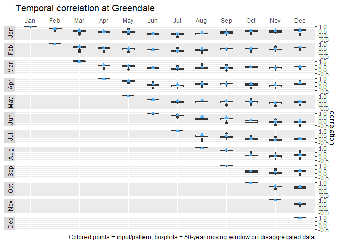
plot(sp_cor)

Temporal Correlation

A final statistic to compare is the monthly cross correlation. This is computed using knnst_temporal_cor() and is only computed for one site at a time. To compute the monthly cross correlation at Greendale:

tmp_cor <- knnst_temporal_cor(disagg, site = "Greendale", bin_size = 50)
plot(tmp_cor)

Recreating Disaggregation

Will be added to vignette

Acknowledgements

This package implements the methods developed by Nowak et al. (2010):

Nowak, K., J. Prairie, B. Rajagopalan, and U. Lall (2010), A nonparametric stochastic approach for multisite disaggregation of annual to daily streamflow, Water Resour. Res., 46, W08529, doi:10.1029/2009WR008530.

It also uses the Meko et al. (2007) paleo reconstructed Lees Ferry natural flow as example data in the package and above:

Meko, D.M., Woodhouse, C.A., Baisan, C.A., Knight, T., Lukas, J.J., Hughes, M.K., and Salzer, M.W. 2007. Medieval Drought in the Upper Colorado River Basin. Geophysical Research Letters 34, L10705.

Disclaimer

This software is in the public domain because it contains materials that originally came from the U.S. Bureau of Reclamation, an agency of the United States Department of Interior.

Although this code has been used by Reclamation, no warranty, expressed or implied, is made by Reclamation or the U.S. Government as to the accuracy and functioning of the program and related program material nor shall the fact of distribution constitute any such warranty, and no responsibility is assumed by Reclamation in connection therewith.

This software is provided “AS IS.”