radhika2026/Daily-Expense-Prediction-and-Analysis-citywise

Analyzed the amount of money being spent every day on transport, food, grocery, etc. also compared cities on the basis of daily expenses. Used the data to predict future expenses.

Daily-Expense-Prediction-and-Analysis-citywise

Analyzed the amount of money being spent every day on transport, food, grocery, etc. also compared cities on the basis of daily expenses. Used the data to predict future expenses.

Objective of the study:

The objective is to answer a series of questions:

1. What percentage of money is spent on groceries, activities, traveling...?
2. What is the preferred public transport?
3. How expensive is each city daily?
4. How much money is spent daily?
5. How much money will be spent in the upcoming days?

Questions 1-4 pseudocode

1. preprocess
2. read data
3. fill empty data 1. date = add year where needed 2. country = get_country_from_city 3. currency = get_currency_from_country 4. currencies
   1. if hrk not set: hrk = lcy * get_rate(currency, 'HRK' date)
   2. if eur not set: eur = hrk * get_rate('HRK', 'EUR', date)
4. plot graphs
5. category - money pie chart
6. public transport pie chart
7. daily city expenses stacked bar chart
8. daily expense bar chart

What about question 5?

how much money will be spent in the upcoming days?

Usually, this would be approached differently; One would try to evalue which machine learning method would be best suitable for adapting to the plotted function. But in this case, we'll pretend to be british empiricists, turn a blind eye and just do the simplest method.

Linear regression pseudocode

1. preprocess
2. convert data into a daily table, with dates and city information
3. encode categorical data
4. avoid the dummy variable trap
5. split data into test and train sets
6. feature scale
7. build our regression model
8. fit the regressor to the train set
9. remove columns that are not beneficial 1. backward elimination
10. predict values
11. plot results

Multiple linear regression

The city column has to be encoded into columns each representing one city.

x = np.array([*zip(range(len(dates)), cities)])
y = sums
from sklearn.preprocessing import OneHotEncoder
from sklearn.compose import ColumnTransformer, make_column_transformer
preprocess = make_column_transformer((OneHotEncoder(), [-1])).fit_transform(x)
x = np.array([*zip(preprocess, x[:, 0])])

Now we have to avoid the dummy variable trap.

x = x[:, 1:]

Next up is to split the data into test and train sets. 80% of the data will be used to train the model, and the rest used for the test set. ytest is the test data we'll compare the regression results to.

from sklearn.model_selection import train_test_split as tts
xtrain, xtest, ytrain, ytest = tts(x, y, test_size = 0.2)

Following the pseudocode the regressor should be created and fit to the training set.

from sklearn.linear_model import LinearRegression
regressor = LinearRegression()
regressor.fit(xtrain, ytrain)

ypred is the list of predicted values using multiple linear regression with all the data available (dates, cities).

ypred = regressor.predict(xtest)

What we could do now is compare the results to the ytest and call it a day. But we're not gonna stop there, let's ask ourselves a question. How beneficial is the abundace of information we're feeding to the regressor? Let's build a quick backward elimination algorithm and let it choose the columns it wants to leave inside. We'll set the p-value to the standard 0.05, sit back, relax, and let the magic unfold.

import statsmodels.formula.api as sm
xopt = np.hstack([np.ones((x.shape[0], 1)), x])
for i in range(xopt.shape[1]):
    pvalues = sm.OLS(y, xopt.astype(np.float64)).fit().pvalues
    mi = np.argmax(pvalues)
    mp = pvalues[mi]
    if mp > 0.05:
        xopt = np.delete(xopt, [mi], 1)
    else:
        break

Now all that's left is to split the data again into test and training sets and get the ypredopt, which is the predicted data of ytest after employing backward elimination.

xtrain, xtest, ytrain, ytest = tts(xopt, y, test_size = 0.2, random_state = 0)
regressor = LinearRegression()
regressor.fit(xtrain, ytrain)

ypredopt = regressor.predict(xtest)

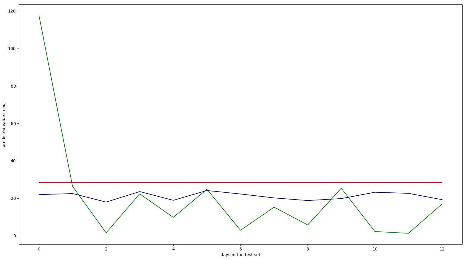
All that's left is to plot everything and check out the result!

plt.plot(ytest, color = 'green')
plt.plot(ypred, color = 'navy')
plt.plot(ypredopt, color = 'red')
plt.ylabel('predicted value in eur')
plt.xlabel('days in the test set')
plt.show()

• green: ytest, real points
• navy/blue: ypred, predicted points before backward elimination
• red: ypredopt, predicted points after backward elimination

Initially the results put me in a spot of bother. The backward elimination threw away all the data altogether. But if we take into consideration the size of the dataset that is logical. The reason that the predicted points before backward elimination are always smaller in this sample is that ytest contains entries only for Poznan, the column on the far left is so high due to weekly shopping.

Cheers!