Credit Card Fraud Simulation using a Non-homogeneous Poisson Process

Intro

The File simulation.py contains all classes necessaries for the simulation. They are:

simulationAssumptions: It handle all assumptions made for the simulation
nonhomogeneous_PoissonProcess: The class responsible for generating arriving times from a non-homogeneous Poisson Process
clients: a class taking care of all clients' info
stores: a class taking care of all stores' info
fraudSimulation: the main class responsible to tie all classes together to run the simulation.

Below I explain the mathematical assumptions made for me to perform the simulation

The simulation model

Consider a city

C = B[0, R'] ⊂ R² ,

with B[0, R'] the closed ball under the norm

|x| = max {x₁, x₂}.

Such city has a population of N clients, a population of N₁ stores of type 1 and, finally, a population of N₂ stores of type 2. Here a store is said to be of type 1 or 2 if

store of type 1 ⇔ the store sells essential goods such as food, gas, ...
store of type 2 ⇔ the store sells nonessential goods such as eletronic gadgets, toys, etc.

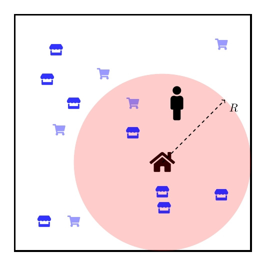
To fix the idea, lets assume the case with only one person in the city, as depicted in the Figure below.

Each person has one house whose position is allocated randomily at the city. Also, it is supposed that there is a radius R > 0 where the person is more likely to be from his/her home. At the same way, stores of type 1 and 2 have their localisation allocated randomily throughout the city.

Now we need to attach the events of payments into this model. This is done with the assistance of the nonhomogeneous Poisson Process.

Let T_n be the time of the nth payment using a credit card (following, as already said, a nonhomogeneous Poisson Process).

At each time T_n we mark with a multinomial random variable Y_n (iid from all others random variables). The random variable Y_n is equivalent to tossing a coin whose values can be either

the nth payment is referent to a product of type 0. Such event happens with probability p0;
or the nth payment is referent to a product of type 1. Such event happens with probability p1;
or a thief is trying to buy a product of type 0 or 1 with a false credit card. Such event happens with probability p2;

(constraint p0 + p1 + p2 == 1)

Finally, the simulation happens in the following manner

wait for a payment time _T_n with a credit card;
toss a coin Y_n;
if the coin is not equal to a fraud then
1. choose randomily a position to a person X. This person X is, also, choosen randomily, and the likelihood of being chosen is in function of his/her credit card limit for the month;
2. choose randomily what kind of product the person X is going to buy. It can be an essentiall good or nonessential;
3. After choosing the type of product the person will choose a store that has a better price and is not that far away from X. In the end, the choise is reduced to a minimization problem where the loss function has as parameters price and distance;
4. Now if the payment doesn't surpass the person's credit card limit then the payment will be tagged as accepted. In case contrary it will be denied the payment and it will be flagged as not accepted.
if the coin is equal to a fraud then
1. choose randomily a position and a person X. This person X will have his/her credit card used for the fraud
2. choose randomily what kind of product is going to buy buy the thieve. It can be an essentiall good or nonessential;
3. Now if the payment doesn't surpass the person's credit card limit then the payment will be tagged as accepted. In case contrary it will be denied the payment and it will be flagged as not accepted;
4. Many more attempts of payments will be done with the same credit card in a small range of time. Such time is given by a geometric distribution with low probabilty;
5. All fraud payments are flagged as fraud;
Continue this process untill the period of time under study is over.

The outcome of the simulation

At the end of the simulation we have a sequence S0, S1, S2, ..., of random variables, saved in a csv file. The csv's rows represent the times a credit card was used and the columns represent the main data desired. The column atributes are:

clientID: client's ID;
buyID: number identificating the credit card payment;
time: time when the payment was done;
moneySpent: amount of money spent;
shop accepted: a boolean value where True means payment accepted anf FALSE otherwise;
was a fraud: a boolean value where True means the payment attempt was comming from a fraud and FALSE otherwise;
store bought from: the ID of the store where the credit card was used;
type product: type of the product bought;
place where cc was used x: x coordinate of the store's place
place where cc was used y: y coordinate of the store's place

How to run the simulation

Given the situation

A city of radius R = 10000km;
A population of 1000 clients;
An amount of 100 stores (summing the ones of type 0 and 1);
A period of 360 days;

We must run at python3

from simulation import *
simulation = fraudSimulation(amount_of_days  = 360,
                             clientsPopSize  = 1_000,
                             storesPopSize   = 100,
                             ball_radius_R   = 10_000)
simulation.runSim()
simulation.print_to_csv('sim.dat')

Then the file sim.dat will have the results of the simulation.

An example obtained after running simulation.py

Setting

simulation = fraudSimulation(amount_of_days  = 360 * 5,
                             clientsPopSize  = 10_000,
                             storesPopSize   = 2_000,
                             ball_radius_R   = 80_000)

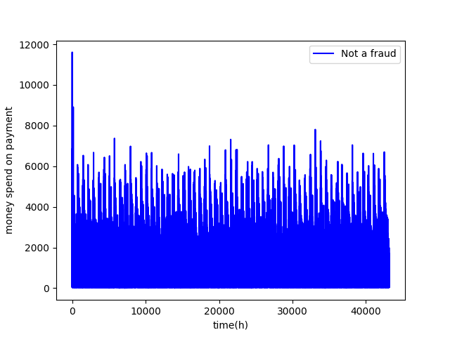
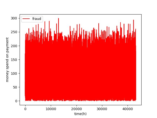
We ended with the following time series

Assumptions

Intensity function

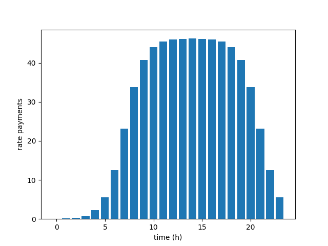
The intensity function for the nonhomogeneous Poisson Process will measure the rate of payments in the period of one day.

The one used by me is a mix of the amount of clients in the simulation and a probability density function. For an amount of 20000 clients, it looks like this