Under the supervision of Prof. Ayon Ganguly,
Department of Mathematics, IIT Guwahati.
Perform regression analysis by:
- Performing point and interval estimation of all parameters
- Testing the significance of the regression
- Conducting residual analysis
- Performing subset selection
- Finding adjusted R2
- Detecting multicollinearity
We have taken the dataset from UC Irvine Machine Learning Repository. The dataset is related to red and white variants of the Portuguese "Vinho Verde" wine. The dataset can be found https://archive.ics.uci.edu/dataset/186/wine+quality.
related research paper can be found https://www.sciencedirect.com/science/article/pii/S0167923609001377?via%3Dihub.
This dataset contains 2 files:
- winequality-red.csv
- winequality-white.csv
we have taken the white wine dataset for our analysis.
The dataset consists of 12 columns and 4898 rows. The columns are as follows:
- fixed acidity
- volatile acidity
- citric acid
- residual sugar
- chlorides
- free sulfur dioxide
- total sulfur dioxide
- density
- pH
- sulphates
- alcohol
- quality
No missing values are present in the dataset. first 5 rows of the dataset are as follows:
| fixed acidity | volatile acidity | citric acid | residual sugar | chlorides | free sulfur dioxide | total sulfur dioxide | density | pH | sulphates | alcohol | quality |
|---|---|---|---|---|---|---|---|---|---|---|---|
| 7.0 | 0.27 | 0.36 | 20.7 | 0.045 | 45.0 | 170.0 | 1.0010 | 3.00 | 0.45 | 8.8 | 6 |
| 6.3 | 0.30 | 0.34 | 1.6 | 0.049 | 14.0 | 132.0 | 0.9940 | 3.30 | 0.49 | 9.5 | 6 |
| 8.1 | 0.28 | 0.40 | 6.9 | 0.050 | 30.0 | 97.0 | 0.9951 | 3.26 | 0.44 | 10.1 | 6 |
| 7.2 | 0.23 | 0.32 | 8.5 | 0.058 | 47.0 | 186.0 | 0.9956 | 3.19 | 0.40 | 9.9 | 6 |
| 7.2 | 0.23 | 0.32 | 8.5 | 0.058 | 47.0 | 186.0 | 0.9956 | 3.19 | 0.40 | 9.9 | 6 |
The analysis of the dataset is as follows:
| Statistic | fixed acidity | volatile acidity | citric acid | residual sugar | chlorides | free sulfur dioxide | total sulfur dioxide | density | pH | sulphates | alcohol | quality |
|---|---|---|---|---|---|---|---|---|---|---|---|---|
| count | 4898.000000 | 4898.000000 | 4898.000000 | 4898.000000 | 4898.000000 | 4898.000000 | 4898.000000 | 4898.000000 | 4898.000000 | 4898.000000 | 4898.000000 | 4898.000000 |
| mean | 6.854788 | 0.278241 | 0.334192 | 6.391415 | 0.045772 | 35.308085 | 138.360657 | 0.994027 | 3.188267 | 0.489847 | 10.514267 | 5.877909 |
| std | 0.843868 | 0.100795 | 0.121020 | 5.072058 | 0.021848 | 17.007137 | 42.498065 | 0.002991 | 0.151001 | 0.114126 | 1.230621 | 0.885639 |
| min | 3.800000 | 0.080000 | 0.000000 | 0.600000 | 0.009000 | 2.000000 | 9.000000 | 0.987110 | 2.720000 | 0.220000 | 8.000000 | 3.000000 |
| 25% | 6.300000 | 0.210000 | 0.270000 | 1.700000 | 0.036000 | 23.000000 | 108.000000 | 0.991723 | 3.090000 | 0.410000 | 9.500000 | 5.000000 |
| 50% | 6.800000 | 0.260000 | 0.320000 | 5.200000 | 0.043000 | 34.000000 | 134.000000 | 0.993740 | 3.180000 | 0.470000 | 10.400000 | 6.000000 |
| 75% | 7.300000 | 0.320000 | 0.390000 | 9.900000 | 0.050000 | 46.000000 | 167.000000 | 0.996100 | 3.280000 | 0.550000 | 11.400000 | 6.000000 |
| max | 14.200000 | 1.100000 | 1.660000 | 65.800000 | 0.346000 | 289.000000 | 440.000000 | 1.038980 | 3.820000 | 1.080000 | 14.200000 | 9.000000 |
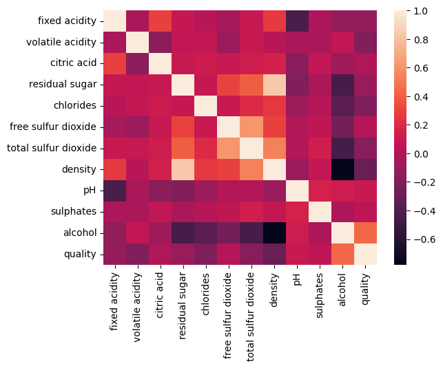
correlation matrix of the dataset is as follows:
| fixed acidity | volatile acidity | citric acid | residual sugar | chlorides | free sulfur dioxide | total sulfur dioxide | density | pH | sulphates | alcohol | quality | |
|---|---|---|---|---|---|---|---|---|---|---|---|---|
| fixed acidity | 1.000000 | -0.022697 | 0.289181 | 0.089021 | 0.023086 | -0.049396 | 0.091070 | 0.265331 | -0.425858 | -0.017143 | -0.120881 | -0.113663 |
| volatile acidity | -0.022697 | 1.000000 | -0.149472 | 0.064286 | 0.070512 | -0.097012 | 0.089261 | 0.027114 | -0.031915 | -0.035728 | 0.067718 | -0.194723 |
| citric acid | 0.289181 | -0.149472 | 1.000000 | 0.094212 | 0.114364 | 0.094077 | 0.121131 | 0.149503 | -0.163748 | 0.062331 | -0.075729 | -0.009209 |
| residual sugar | 0.089021 | 0.064286 | 0.094212 | 1.000000 | 0.088685 | 0.299098 | 0.401439 | 0.838966 | -0.194133 | -0.026664 | -0.450631 | -0.097577 |
| chlorides | 0.023086 | 0.070512 | 0.114364 | 0.088685 | 1.000000 | 0.101392 | 0.198910 | 0.257211 | -0.090439 | 0.016763 | -0.360189 | -0.209934 |
| free sulfur dioxide | -0.049396 | -0.097012 | 0.094077 | 0.299098 | 0.101392 | 1.000000 | 0.615501 | 0.294210 | -0.000618 | 0.059217 | -0.250104 | 0.008158 |
| total sulfur dioxide | 0.091070 | 0.089261 | 0.121131 | 0.401439 | 0.198910 | 0.615501 | 1.000000 | 0.529881 | 0.002321 | 0.134562 | -0.448892 | -0.174737 |
| density | 0.265331 | 0.027114 | 0.149503 | 0.838966 | 0.257211 | 0.294210 | 0.529881 | 1.000000 | -0.093591 | 0.074493 | -0.780138 | -0.307123 |
| pH | -0.425858 | -0.031915 | -0.163748 | -0.194133 | -0.090439 | -0.000618 | 0.002321 | -0.093591 | 1.000000 | 0.155951 | 0.121432 | 0.099427 |
| sulphates | -0.017143 | -0.035728 | 0.062331 | -0.026664 | 0.016763 | 0.059217 | 0.134562 | 0.074493 | 0.155951 | 1.000000 | -0.017433 | 0.053678 |
| alcohol | -0.120881 | 0.067718 | -0.075729 | -0.450631 | -0.360189 | -0.250104 | -0.448892 | -0.780138 | 0.121432 | -0.017433 | 1.000000 | 0.435575 |
| quality | -0.113663 | -0.194723 | -0.009209 | -0.097577 | -0.209934 | 0.008158 | -0.174737 | -0.307123 | 0.099427 | 0.053678 | 0.435575 | 1.000000 |
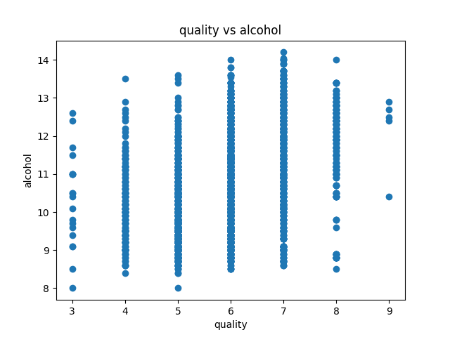
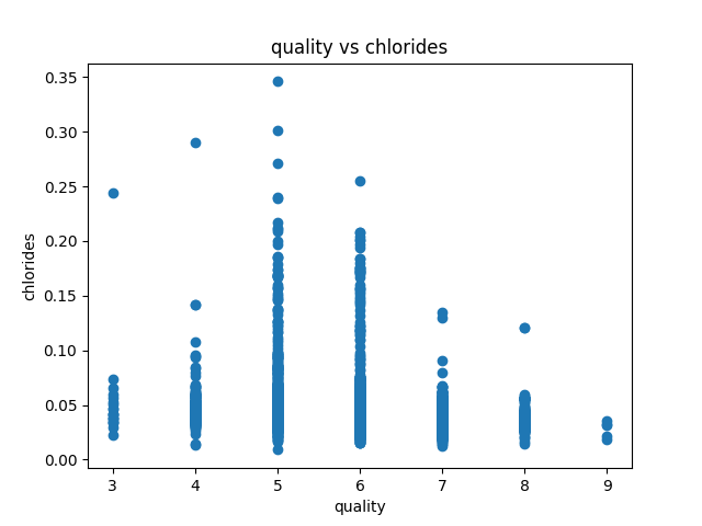
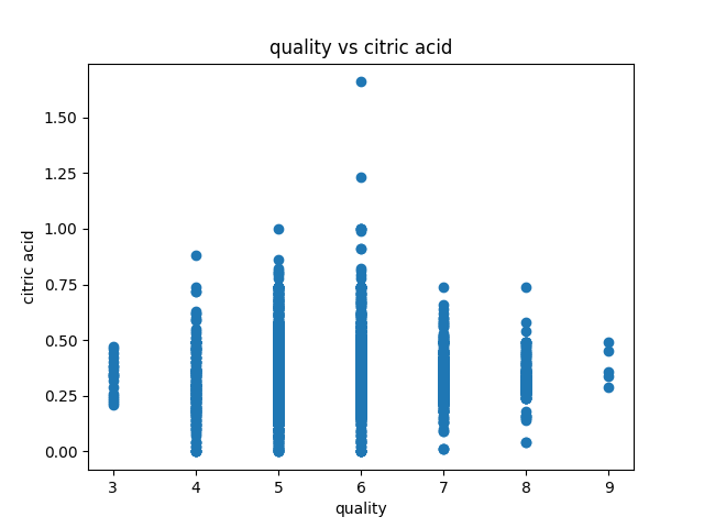
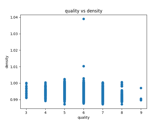
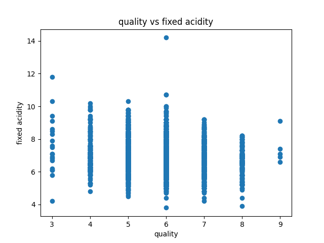
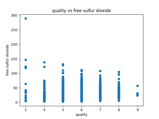
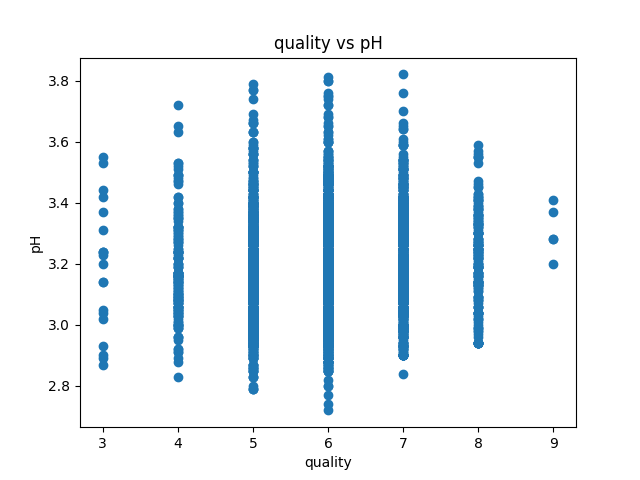
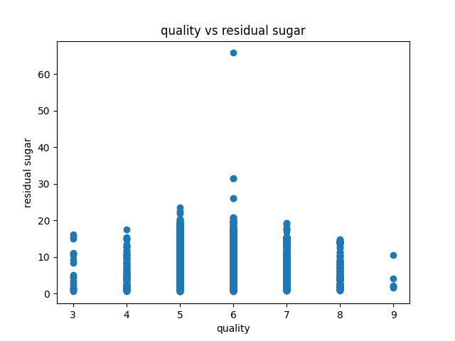
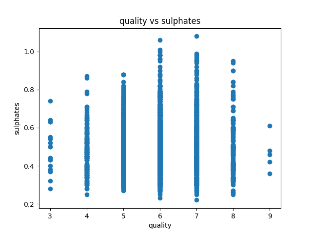
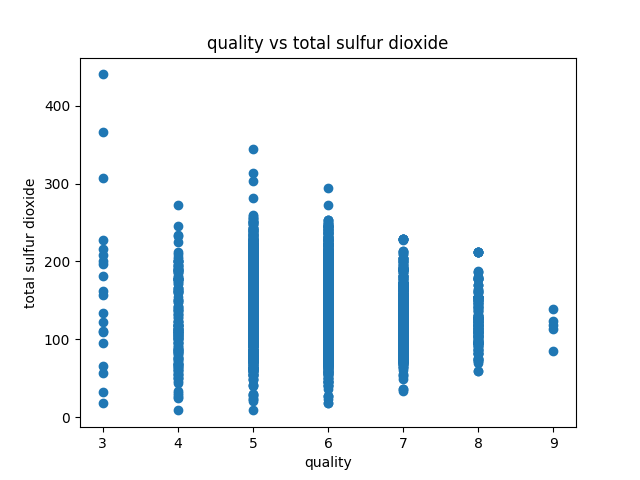
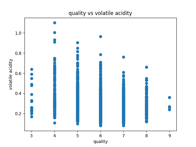
Data visualization of the dataset is as follows:
correlation matrix plot of the dataset is as follows:we have considered the quality of the wine as the dependent variable and all other variables as independent variables. Now we have fitted a multiple linear regression model to the dataset using scikit-learn for estimating the parameters.
it uses the normal equation for estimating the parameters internally.
where
The estimated parameters are as follows:
We estimate the confidence intervals of the parameters using the given formula:
where
The confidence intervals of the parameters are as follows:
For estimating the confidence intervals of the parameters, we have used statsmodels library.
We have tested the significance of the regression using the F-test. The null hypothesis is that all the parameters are zero. The alternative hypothesis is that at least one parameter is non-zero. The F-statistic is calculated as follows:
where
Conclusion: At least one independent variable is contributing to the explanation of the dependent variable.
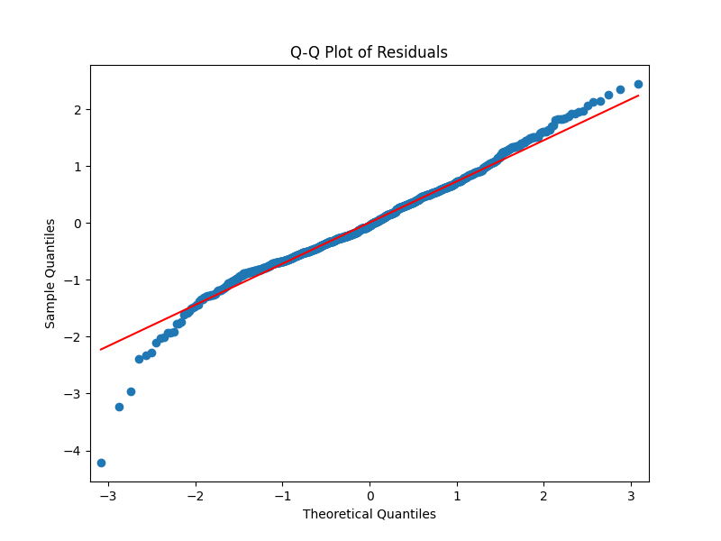
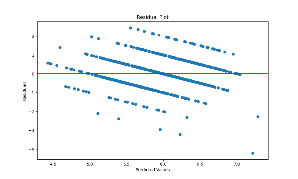
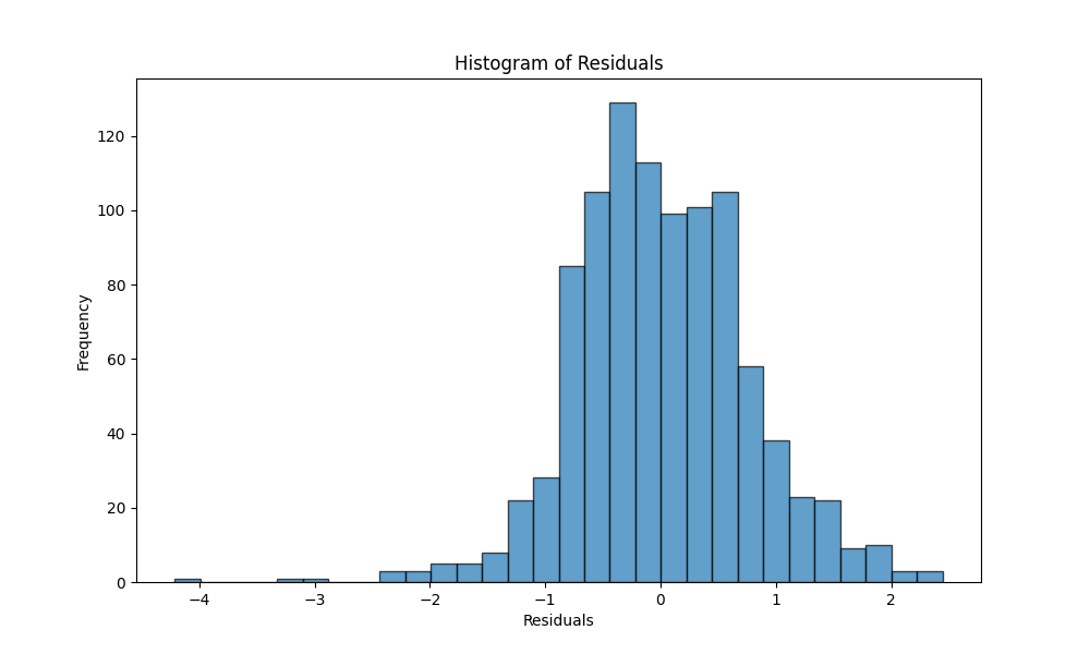
We have divided the dataset into training and testing datasets. We have fitted the model to the training dataset and predicted the values of the testing dataset. The residuals are calculated as the difference between the actual values and the predicted values. The residuals are plotted against the predicted values. The residuals are normally distributed as we can see in the Q-Q plot and the other plots. The residuals are plotted against the predicted values.
The adjusted R2 is calculated as follows:
where
where
Among the large number of possible explanatory variables, we wish to select those which explain the observed responses the best. This way, we can decrease the number of predictors (giving a parsimonious model) and get good predictive power by eliminating redundant variables. In this section, we briefly present three methods for variable selection.
The forward selection method is an iterative method. In the first iteration we consider
which feature f1 is the most significant in terms of its P-value for the F-test with f1 ∈
From this procedure we get: ['alcohol', 'volatile acidity', 'residual sugar', 'free sulfur dioxide', 'density', 'pH', 'sulphates', 'fixed acidity']
This time, we start with the complete model and at each step, we delete the variable with lowest value of Student’s test statistic (largest P-value) in absolute value, as long as it is not significant (at a specified level
From this procedure we get: ['fixed acidity', 'volatile acidity', 'residual sugar', 'free sulfur dioxide', 'density', 'pH', 'sulphates', 'alcohol']
- Start with an Empty Model or Full Model:
- You can start with either an empty model (no predictors) or a full model (all predictors included).
- Iterate:
- Perform both forward selection and backward elimination iteratively.
- At each step, evaluate whether adding or removing a predictor variable improves the model based on the chosen criterion.
- Stop the iteration when no further improvement is observed or when predefined stopping criteria are met (e.g., no variables meet the criteria for inclusion or removal).
From this procedure we get: ['alcohol', 'volatile acidity', 'residual sugar', 'free sulfur dioxide', 'density', 'pH', 'sulphates', 'fixed acidity']
-
Introduction Multicollinearity is a phenomenon in regression analysis where independent variables are highly correlated with each other, which can impact the interpretation and reliability of regression results.
-
Multicollinearity Assessment The Variance Inflation Factor (VIF) was employed to assess multicollinearity among the independent variables in the regression model.
where
This measures the factor by which the variance of
VIF values above a certain threshold (commonly 10) indicate multicollinearity.
Highlight any variables with high VIF values, indicating strong collinearity with other variables in the model
- Results The following table displays the VIF values for each independent variable:
| Variable | VIF Value |
|---|---|
| fixed acid | 92.86 |
| volatile acidity | 9.730 |
| citric acid | 10.01 |
| residual sugar | 3.830 |
| ... | ... |
Variables with VIF values exceeding the threshold of 10 indicate multicollinearity, suggesting strong correlations with other variables in the model.
-
Discussion Multicollinearity can lead to inflated standard errors, unreliable hypothesis tests, and challenges in interpreting regression coefficients.
-
Conclusion The assessment of multicollinearity underscores its importance in regression analysis. Strategies for addressing multicollinearity, such as dropping highly correlated variables or using regularization techniques, may be necessary to ensure the reliability of regression results.
