teamcolors

An R package providing color palettes for pro and amateur sports teams. The palettes are provided by Jim Neilsen’s Team Colors website and offered with only minimal alterations. NCAA colors come from teamcolorcodes.com, via the ncaahoopR package.

Install

To install the CRAN version, use:

install.packages(teamcolors)

To install the development version from GitHub, use:

devtools::install_github("beanumber/teamcolors")

Load

library(teamcolors)
head(teamcolors)

## # A tibble: 6 x 11
##   name  league primary secondary tertiary quaternary division location mascot
##   <chr> <chr>  <chr>   <chr>     <chr>    <chr>      <chr>    <chr>    <chr> 
## 1 A&M-… ncaa   #0067C5 #007F3E   <NA>     <NA>       Southla… A&M-Cor… Chris…
## 2 Abil… ncaa   #461D7C #FFFFFF   <NA>     <NA>       Southla… Abilene  Chris…
## 3 AFC … epl    #e62333 #000000   <NA>     <NA>       <NA>     AFC      Bourn…
## 4 Air … ncaa   #003087 #8A8D8F   #B1B3B3  #FFC72C    MWC      Air For… <NA>  
## 5 Akro… ncaa   #041E42 #A89968   <NA>     <NA>       MAC      Akron    Zips  
## 6 Alab… ncaa   #660000 #FFFFFF   <NA>     <NA>       SWAC     Alabama  A&M   
## # … with 2 more variables: sportslogos_name <chr>, logo <chr>

Show palettes

Sometimes you need to work with a named vector of colors. Other times you can use the built-in scale_color_teams() and scale_color_fill() functions.

league_pal("nba")

##          Atlanta Hawks         Boston Celtics          Brooklyn Nets 
##              "#e13a3e"              "#008348"              "#061922" 
##      Charlotte Hornets          Chicago Bulls    Cleveland Cavaliers 
##              "#1d1160"              "#ce1141"              "#860038" 
##       Dallas Mavericks         Denver Nuggets        Detroit Pistons 
##              "#007dc5"              "#4d90cd"              "#ed174c" 
##  Golden State Warriors        Houston Rockets         Indiana Pacers 
##              "#fdb927"              "#ce1141"              "#ffc633" 
##   Los Angeles Clippers     Los Angeles Lakers      Memphis Grizzlies 
##              "#ed174c"              "#fdb927"              "#0f586c" 
##             Miami Heat        Milwaukee Bucks Minnesota Timberwolves 
##              "#98002e"              "#00471b"              "#005083" 
##   New Orleans Pelicans        New York Knicks  Oklahoma City Thunder 
##              "#002b5c"              "#006bb6"              "#007dc3" 
##          Orlando Magic     Philadelphia 76ers           Phoenix Suns 
##              "#007dc5"              "#ed174c"              "#e56020" 
## Portland Trail Blazers       Sacramento Kings      San Antonio Spurs 
##              "#e03a3e"              "#724c9f"              "#bac3c9" 
##        Toronto Raptors              Utah Jazz     Washington Wizards 
##              "#ce1141"              "#002b5c"              "#002b5c"

Plot

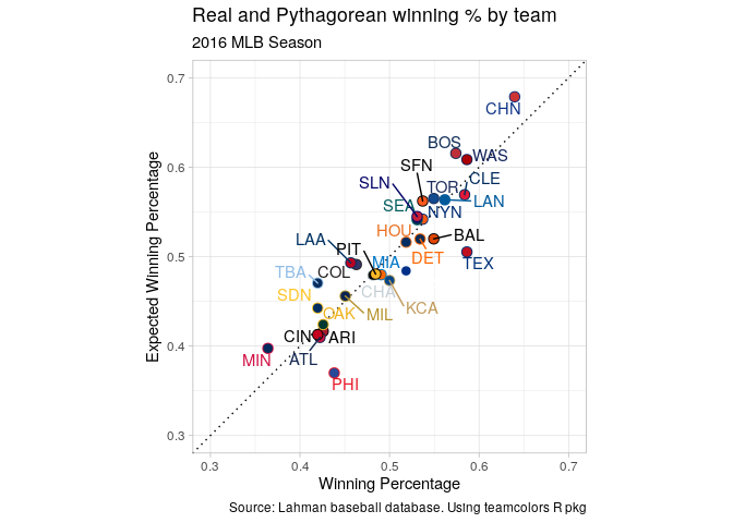
In baseball, Pythagorean expectation relates expected winning percentage to runs allowed and runs scored. How well does it work?

library(Lahman)
library(tidyverse)
pythag <- Teams %>%
  filter(yearID == 2016) %>%
  select(name, teamID, yearID, W, L, R, RA) %>%
  mutate(
    wpct = W / (W + L), exp_wpct = 1 / (1 + (RA / R)^2),
    # note name discrepancy!
    name = ifelse(name == "Los Angeles Angels of Anaheim", "Los Angeles Angels", name)
  )

`ggplot2`

ggplot(pythag, aes(x = wpct, y = exp_wpct, color = name, fill = name)) +
  geom_abline(slope = 1, intercept = 0, linetype = 3) +
  geom_point(shape = 21, size = 3) +
  scale_fill_teams(guide = FALSE) +
  scale_color_teams(2, guide = FALSE) +
  ggrepel::geom_text_repel(aes(label = teamID)) +
  scale_x_continuous("Winning Percentage", limits = c(0.3, 0.7)) +
  scale_y_continuous("Expected Winning Percentage", limits = c(0.3, 0.7)) +
  theme_light() +
  labs(
    title = "Real and Pythagorean winning % by team",
    subtitle = paste(first(pull(pythag, yearID)), "MLB Season", sep = " "),
    caption = "Source: Lahman baseball database. Using teamcolors R pkg"
  ) +
  coord_equal()

Base R

pythag <- pythag %>%
  left_join(teamcolors, by = "name")
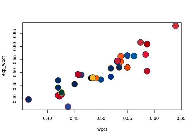
with(pythag, plot(wpct, exp_wpct, bg = primary, col = secondary, pch = 21, cex = 3))

Key

You can see the color palettes using existing functionality from the scales package, but it won’t show the names of the teams.

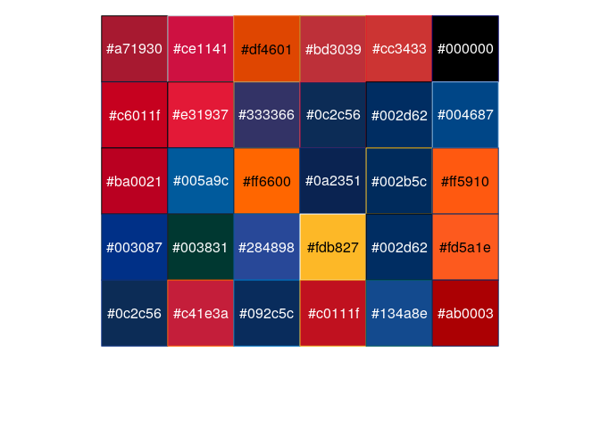
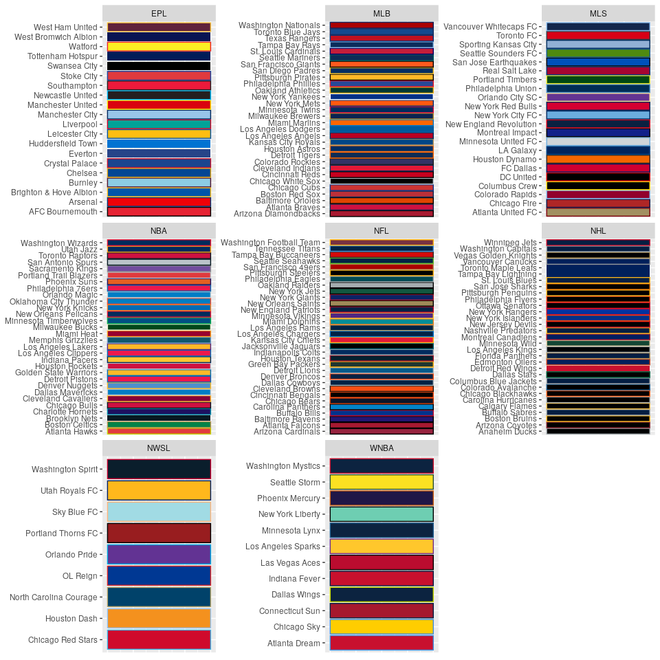
scales::show_col(league_pal("mlb"), borders = league_pal("mlb", 2))

So, instead, use show_team_col(). Note that this only shows color palettes for non-NCAA teams.

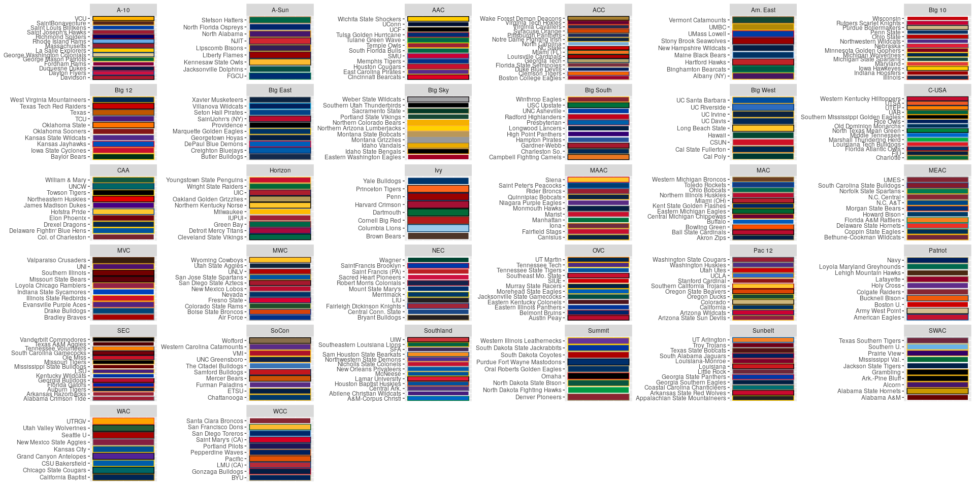
show_team_col()

To view color palettes for college teams, use the show_ncaa_col() function.

show_ncaa_col()

Logos

Links to team logos are provided by (http://www.sportslogos.net/).

teamcolors %>%
  filter(grepl("New ", name)) %>%
  pull(logo) %>%
  knitr::include_graphics()

Note that we don’t have any coverage for the EPL.

teamcolors %>%
  group_by(league) %>%
  summarize(
    num_teams = n(),
    num_logos = sum(!is.na(logo))
  )

## `summarise()` ungrouping output (override with `.groups` argument)

## # A tibble: 9 x 3
##   league num_teams num_logos
##   <chr>      <int>     <int>
## 1 epl           20         0
## 2 mlb           30        30
## 3 mls           22        22
## 4 nba           30        30
## 5 ncaa         353       301
## 6 nfl           32        31
## 7 nhl           31        31
## 8 nwsl           9         8
## 9 wnba          12        12

References

For more examples see:

Lopez, M.J., Matthews, G.J., Baumer, B.S., “How often does the best team win? A unified approach to understanding randomness in North American sport,” The Annals of Applied Statistics, vol. 12, no. 4, 2018, pp. 2483–2516. URL (https://projecteuclid.org/euclid.aoas/1542078053)

To cite this package in your work, see:

citation("teamcolors")

ransomts/teamcolors