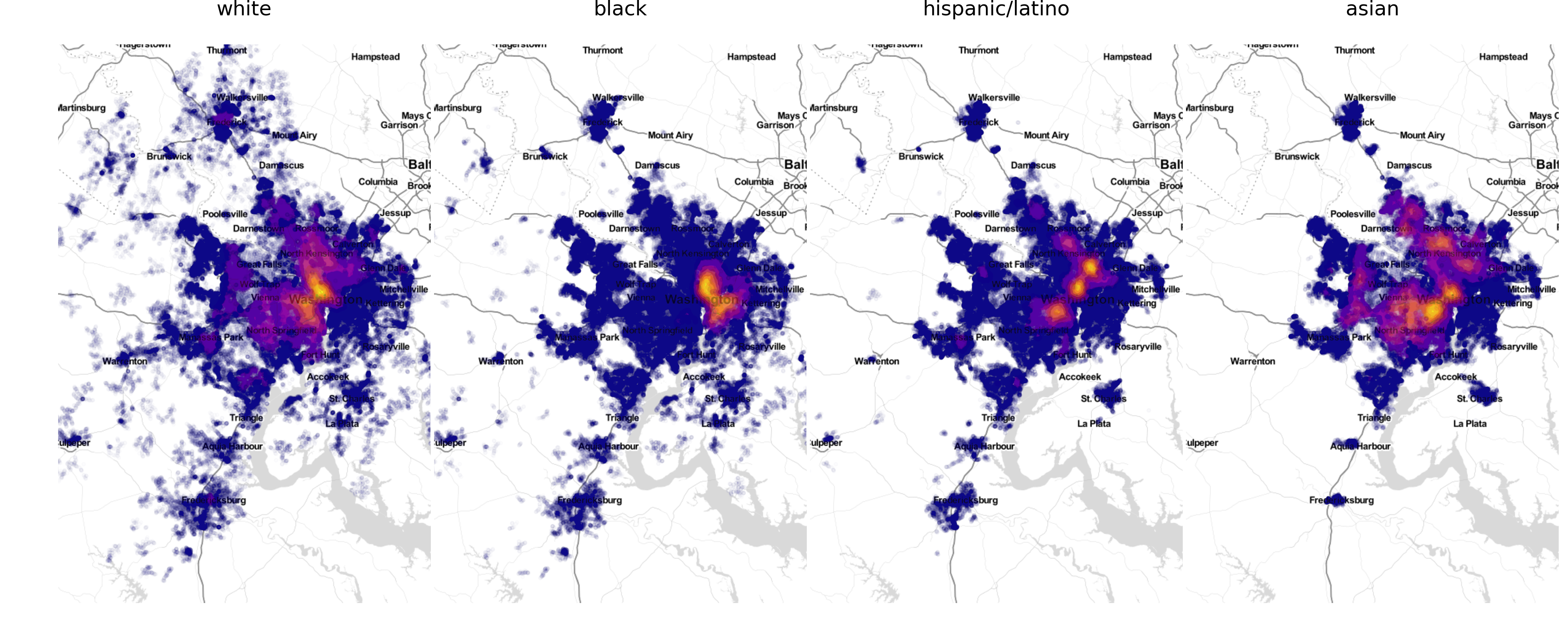
The PySAL segregation package is a tool for analyzing patterns of urban segregation. With only a few lines of code, segregation users can
Calculate over 40 segregation measures from simple to state-of-the art, including:
- aspatial segregation indices
- spatial segregation indices
- local segregation indices
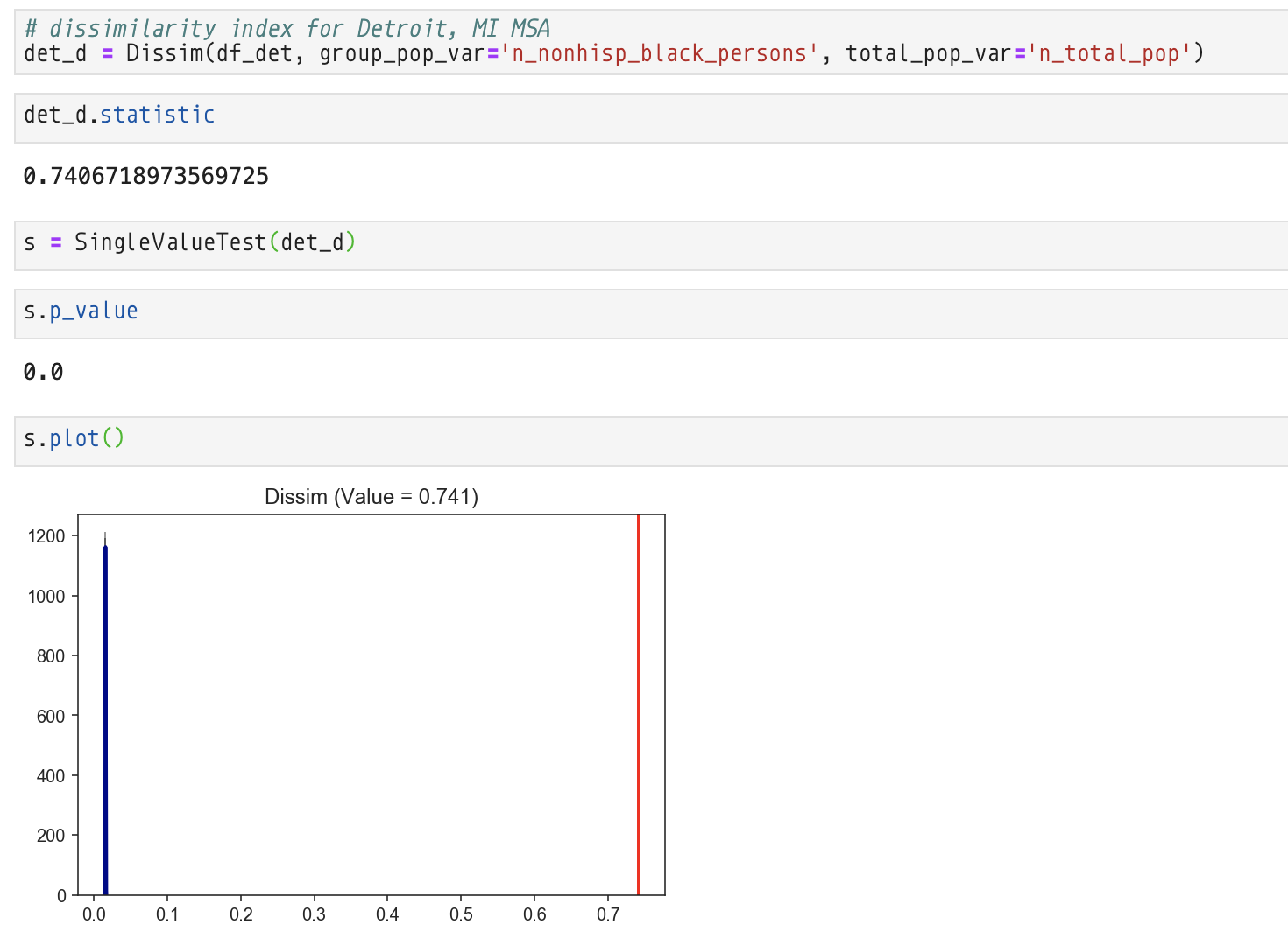
Test whether segregation estimates are statistically significant:
Decompose segregation comparisons into
- differences arising from spatial structure
- differences arising from demographic structure
Released versions of segregation are available on pip and anaconda
pip:
pip install segregationconda install -c conda-forge segregationYou can also install the current development version from this repository
download anaconda:
cd into the directory and run the following commands
conda env create -f environment.yml
conda activate segregation
python setup.py developFor a complete guide to the segregation API, see the online
documentation.
For code walkthroughs and sample analyses, see the example notebooks
Each index in the segregation module is implemented as a class, which is built from a pandas.DataFrame
or a geopandas.GeoDataFrame. To estimate a segregation statistic, a user needs to call the segregation class
she wishes to estimate, and pass three arguments:
- the DataFrame containing population data
- the name of the column with population counts for the group of interest
- the name of the column with the total population for each enumeration unit
Every class in segregation has a statistic and a core_data attributes.
The first is a direct access to the point estimation of the specific segregation measure
and the second attribute gives access to the main data that the module uses internally to
perform the estimates.
If, for example, a user was studying income segregation and wanted to know whether
high-income residents tend to be more segregated from others.
This user may want would want to fit a dissimilarity index (D) to a DataFrame called df to
a specific group with columns like "hi_income", "med_income" and "low_income" that store counts of people in each income
bracket, and a total column called "total_population". A typical call would be something like this:
from segregation.aspatial import Dissim
d_index = Dissim(df, "hi_income", "total_population")
To see the estimated D in the first generic example above, the user would have just to run
d_index.statistic to see the fitted value.
If a user would want to fit a spatial dissimilarity index (SD), the call would be nearly
identical, save for the fact that the DataFrame now needs to be a GeoDataFrame with an appropriate geometry column
from segregation.spatial import SpatialDissim
spatial_index = SpatialDissim(gdf, "hi_income", "total_population")
Some spatial indices can also accept either a PySAL W object, or a pandana Network object,
which allows the user full control over how to parameterize spatial effects.
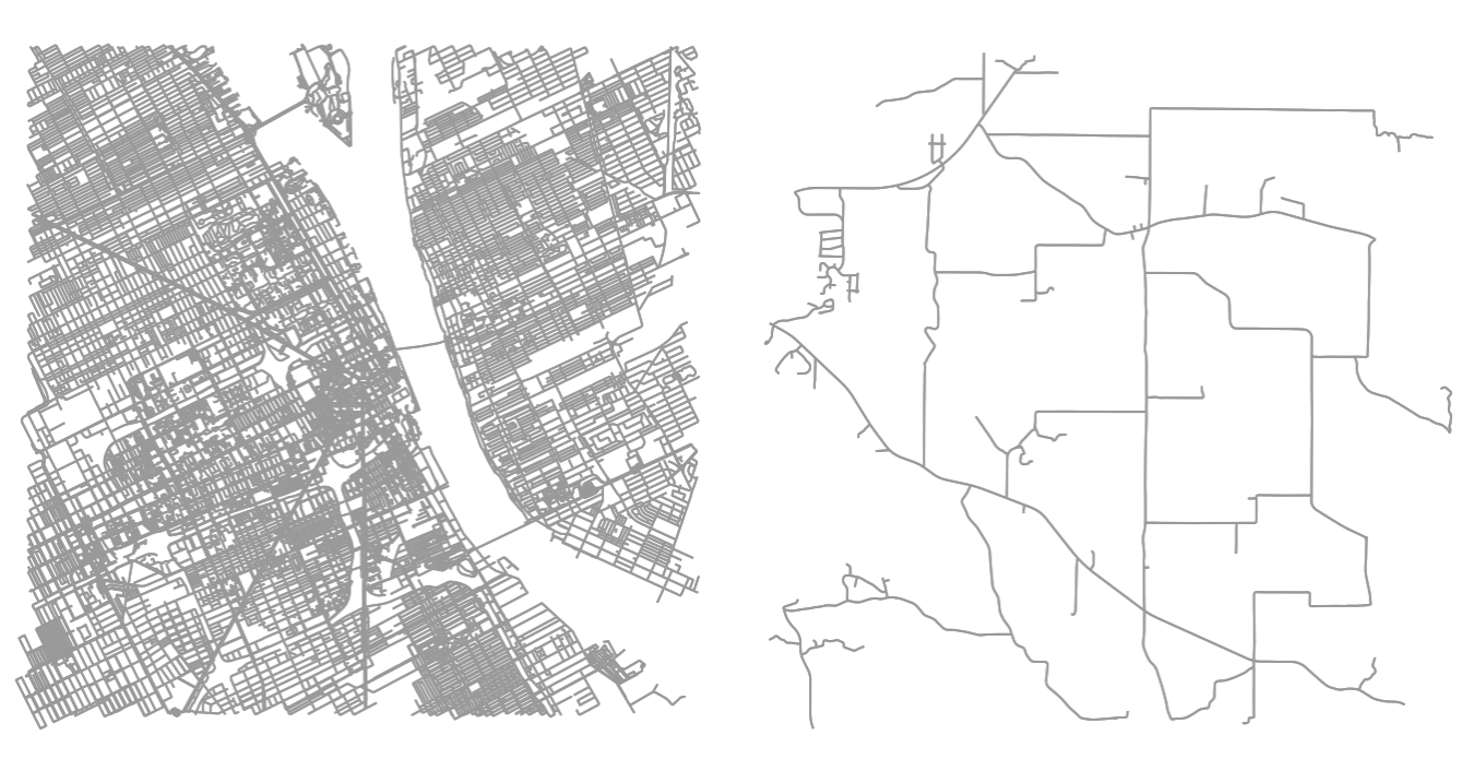
The network functions can be particularly useful for teasing out differences in
segregation measures caused by two cities that have two very different spatial structures,
like for example Detroit MI (left) and Monroe LA (right):
For point estimation, all single-group indices available are summarized in the following table:
| Measure | Class/Function | Spatial? | Specific Arguments |
|---|---|---|---|
| Dissimilarity (D) | Dissim | No | - |
| Gini (G) | GiniSeg | No | - |
| Entropy (H) | Entropy | No | - |
| Isolation (xPx) | Isolation | No | - |
| Exposure (xPy) | Exposure | No | - |
| Atkinson (A) | Atkinson | No | b |
| Correlation Ratio (V) | CorrelationR | No | - |
| Concentration Profile (R) | ConProf | No | m |
| Modified Dissimilarity (Dct) | ModifiedDissim | No | iterations |
| Modified Gini (Gct) | ModifiedGiniSeg | No | iterations |
| Bias-Corrected Dissimilarity (Dbc) | BiasCorrectedDissim | No | B |
| Density-Corrected Dissimilarity (Ddc) | DensityCorrectedDissim | No | xtol |
| Minimun-Maximum Index (MM) | MinMax | No | |
| Spatial Proximity Profile (SPP) | SpatialProxProf | Yes | m |
| Spatial Dissimilarity (SD) | SpatialDissim | Yes | w, standardize |
| Boundary Spatial Dissimilarity (BSD) | BoundarySpatialDissim | Yes | standardize |
| Perimeter Area Ratio Spatial Dissimilarity (PARD) | PerimeterAreaRatioSpatialDissim | Yes | standardize |
| Distance Decay Isolation (DDxPx) | DistanceDecayIsolation | Yes | alpha, beta, metric |
| Distance Decay Exposure (DDxPy) | DistanceDecayExposure | Yes | alpha, beta, metric |
| Spatial Proximity (SP) | SpatialProximity | Yes | alpha, beta, metric |
| Absolute Clustering (ACL) | AbsoluteClustering | Yes | alpha, beta, metric |
| Relative Clustering (RCL) | RelativeClustering | Yes | alpha, beta, metric |
| Delta (DEL) | Delta | Yes | - |
| Absolute Concentration (ACO) | AbsoluteConcentration | Yes | - |
| Relative Concentration (RCO) | RelativeConcentration | Yes | - |
| Absolute Centralization (ACE) | AbsoluteCentralization | Yes | - |
| Relative Centralization (RCE) | RelativeCentralization | Yes | - |
| Relative Centralization (RCE) | RelativeCentralization | Yes | - |
| Spatial Minimun-Maximum (SMM) | SpatialMinMax | Yes | network, w, decay, distance, precompute |
segregation also facilitates the estimation of multigroup segregation measures.
In this case, the call is nearly identical to the single-group, only now we pass a list of column names rather than a single string; reprising the income segregation example above, an example call might look like this
from segregation.aspatial import MultiDissim
index = MultiDissim(df, ['hi_income', 'med_income', 'low_income'])index.statisticAvailable multi-group indices are summarized in the table below:
| Measure | Class/Function | Spatial? | Specific Arguments |
|---|---|---|---|
| Multigroup Dissimilarity | MultiDissim | No | - |
| Multigroup Gini | MultiGiniSeg | No | - |
| Multigroup Normalized Exposure | MultiNormalizedExposure | No | - |
| Multigroup Information Theory | MultiInformationTheory | No | - |
| Multigroup Relative Diversity | MultiRelativeDiversity | No | - |
| Multigroup Squared Coefficient of Variation | MultiSquaredCoefficientVariation | No | - |
| Multigroup Diversity | MultiDiversity | No | normalized |
| Simpson’s Concentration | SimpsonsConcentration | No | - |
| Simpson’s Interaction | SimpsonsInteraction | No | - |
| Multigroup Divergence | MultiDivergence | No | - |
Also, it is possible to calculate local measures of segregation.
A statistics attribute will contain the values of these indexes. Note:
in this case the attribute is in the plural since, many statistics are fitted, one for
each enumeration unit Local segregation indices have the same signature as their global
cousins and are summarized in the table below:
| Measure | Class/Function | Spatial? | Specific Arguments |
|---|---|---|---|
| Location Quotient | MultiLocationQuotient | No | - |
| Local Diversity | MultiLocalDiversity | No | - |
| Local Entropy | MultiLocalEntropy | No | - |
| Local Simpson’s Concentration | MultiLocalSimpsonConcentration | No | - |
| Local Simpson’s Interaction | MultiLocalSimpsonInteraction | No | - |
| Local Centralization | LocalRelativeCentralization | Yes | - |
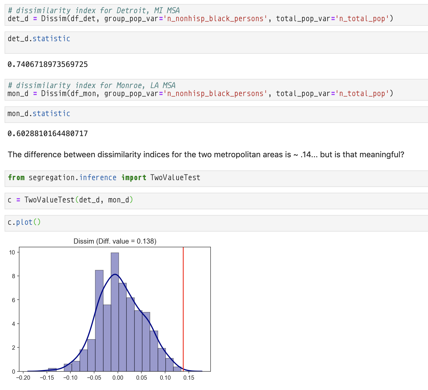
Once the segregation indexes are fitted, the user can perform inference to shed light for statistical significance in regional analysis. The summary of the inference framework is presented in the table below:
| Inference Type | Class/Function | Function main Inputs | Function Outputs |
|---|---|---|---|
| Single Value | SingleValueTest | seg_class, iterations_under_null, null_approach, two_tailed | p_value, est_sim, statistic |
| Two Values | TwoValueTest | seg_class_1, seg_class_2, iterations_under_null, null_approach | p_value, est_sim, est_point_diff |
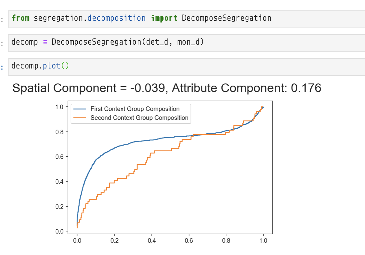
Another useful analysis that can be performed with the segregation module is a
decompositional approach where two different indexes can be broken down into their spatial
component (c_s) and attribute component (c_a). This framework is summarized in the table
below:
| Framework | Class/Function | Function main Inputs | Function Outputs |
|---|---|---|---|
| Decomposition | DecomposeSegregation | index1, index2, counterfactual_approach | c_a, c_s |
In this case, the difference in measured D statistics between Detroit and Monroe is attributable primarily to their demographic makeup, rather than the spatial structure of the two cities. (Note, this is to be expected since D is not a spatial index)
PySAL-segregation is under active development and contributors are welcome.
If you have any suggestion, feature request, or bug report, please open a new issue on GitHub. To submit patches, please follow the PySAL development guidelines and open a pull request. Once your changes get merged, you’ll automatically be added to the Contributors List.
If you are having issues, please talk to us in the gitter room.
The project is licensed under the BSD license.
 Award #1831615
RIDIR: Scalable Geospatial Analytics for Social Science Research
 Renan Xavier Cortes is grateful for the support of Coordenação de Aperfeiçoamento de
Pessoal de Nível Superior - Brazil (CAPES) - Process number 88881.170553/2018-01
