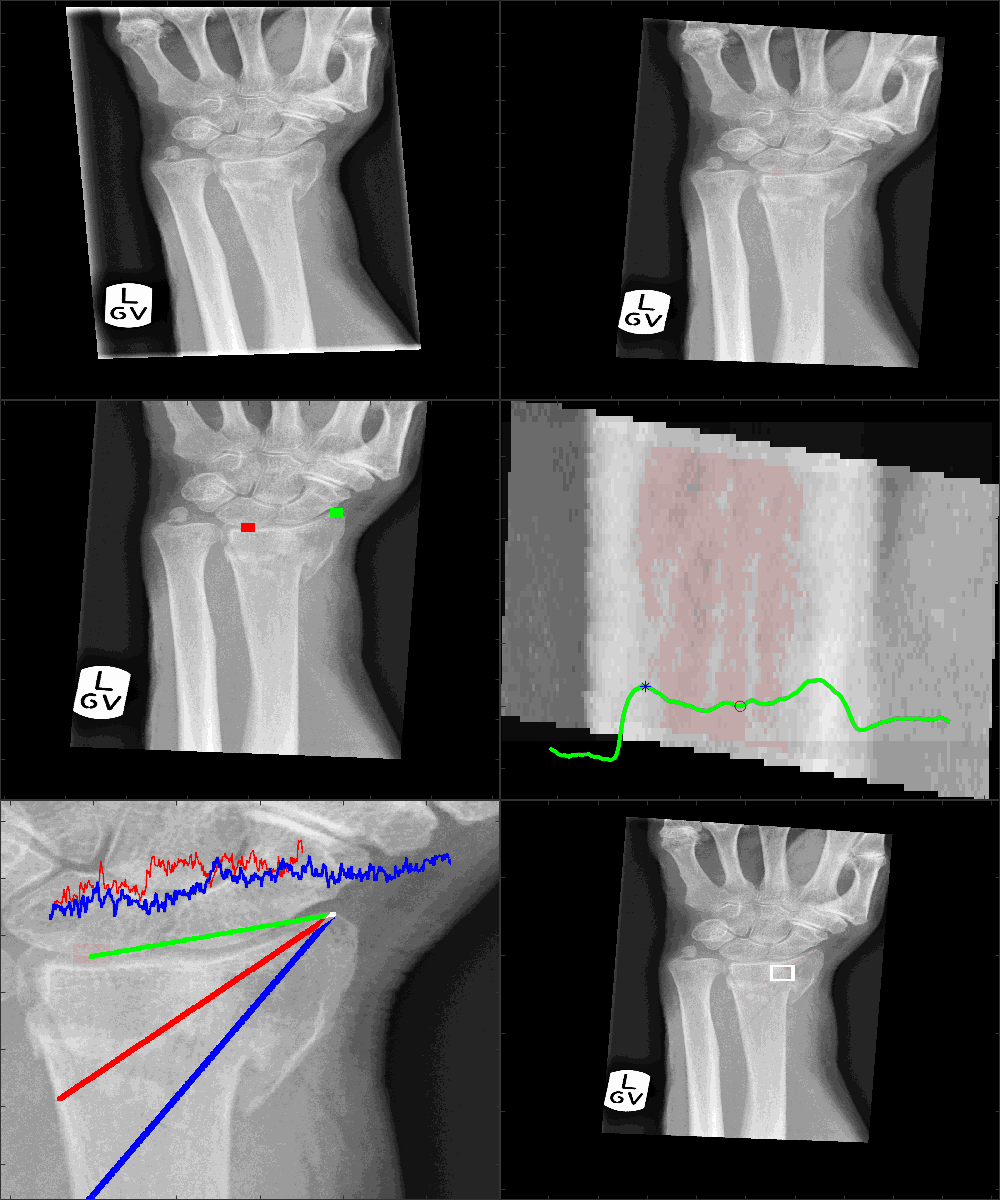
This repository describes a semi-automatic image processing algorithm for the geometric analysis of dorsally displaced wrist fractures (Colles’ fractures). The semi-automatic analysis require the manual location of three landmarks (finger, lunate and radial styloid) and automatic processing to generate 32 geometric and texture measurements, which may be related to conditions such as osteoporosis and swelling of the wrist.
This work has been published in PLOS ONE, if you find the work or the software interesting or useful, please cite as:
Reyes-Aldasoro CC, Ngan KH, Ananda A, d’Avila Garcez A, Appelboam A, Knapp KM (2020) Geometric semi-automatic analysis of radiographs of Colles’ fractures. PLoS ONE 15(9): e0238926. https://doi.org/10.1371/journal.pone.0238926
A previous version of this paper was submitted to MedRXiv (https://www.medrxiv.org/content/10.1101/2020.02.18.20024562v1)
Fractures of the wrist are common in Emergency Departments, where some patients are treated with a procedure called Manipulation under Anaesthesia. In some cases this procedure is unsuccessful and patients need to visit the hospital again where they undergo surgery to treat the fracture. This work describes a geometric semi-automatic image analysis algorithm to analyse and compare the x-rays of healthy controls and patients with dorsally displaced wrist fractures (Colles' fractures) who were treated with Manipulation under Anaesthesia.
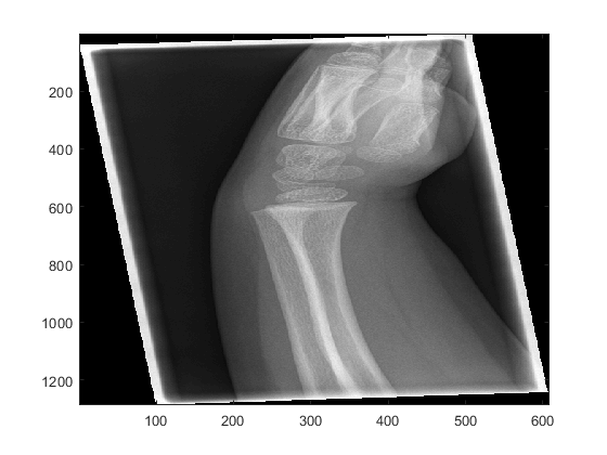
If your data is in DICOM format, you can read into Matlab using the functions dicomread and dicominfo like this
dicom_header = dicominfo('D:\IMG0');
dicom_image = dicomread('D:\IMG0');
dicom_header
dicom_header =
struct with fields:
                            Filename: 'D:\IMG0'
                         FileModDate: '27-Jun-2017 11:19:50'
                            FileSize: 1567164
                              Format: 'DICOM'
                       FormatVersion: 3
                               Width: 608
                              Height: 1287
                            BitDepth: 12
                           ColorType: 'grayscale'
                           .
                           .
                           .
           PhotometricInterpretation: 'MONOCHROME2'
                                Rows: 1287
                             Columns: 608
imagesc(dicom_image)
colormap gray
If you are going to handle numerous images, it can be convenient to read the dicom and then save in Matlab format as a .mat file. You can save the header and the image into a single file. In subsequent files, the image will be identified with the name "Xray" and the header with the name "Xray_info". Later on you can also add the mask (the three landmarks) as "Xray_mask". Then these can be loaded together from one file, e.g.
clear load('D:\PATIENT_PA.mat')whos
  Name              Size                 Bytes  Class     Attributes
Xray           2500x2048            40960000  double

Xray_info         1x1                  16820  struct

Xray_mask      2500x2048            40960000  double
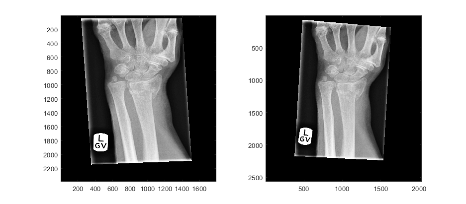
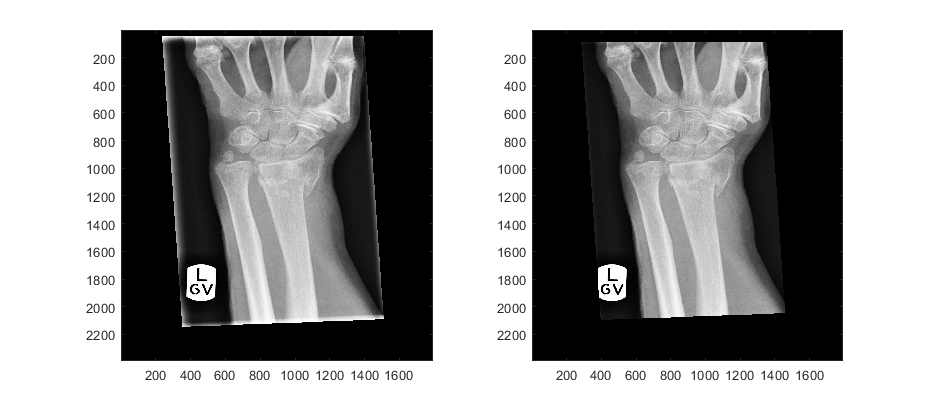
To rotate the Xray so that the forearm is aligned vertically, use the function alingXray. If you are already using a mask, the mask should also be b provided so that it is rotated with the same angle. The actual angle of rotation is one output parameter.
[XrayR,Xray_maskR,angleRot] = alignXray (Xray,Xray_mask);disp(angleRot)
figure(1) subplot(121) imagesc(Xray) subplot(122) imagesc(XrayR)
-13
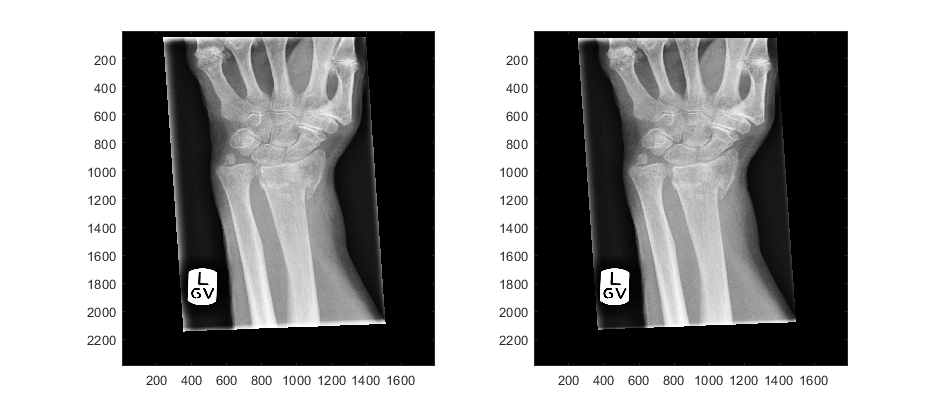
In case the image has lines due to the collimator and these should be removed, use the function removeEdgesCollimator. The function receives the Xray as input, and if desired a second parameter that controls the width of the removal, if the default value (set at 25) does not work, try increasing it.
load('D:\OneDrive - City, University of London\Acad\Research\Exeter_Fracture\DICOM_Karen\ANON8949_PATIENT_PA_594.mat')XrayR2 = removeEdgesCollimator2(Xray); figure(1) subplot(121) imagesc(Xray) subplot(122) imagesc(XrayR2)
XrayR2 = removeEdgesCollimator2(Xray,70); figure(2) subplot(121) imagesc(Xray) subplot(122) imagesc(XrayR2) colormap gray
Notice that we are concatenating results: Xray -> XrayR -> XrayR2.
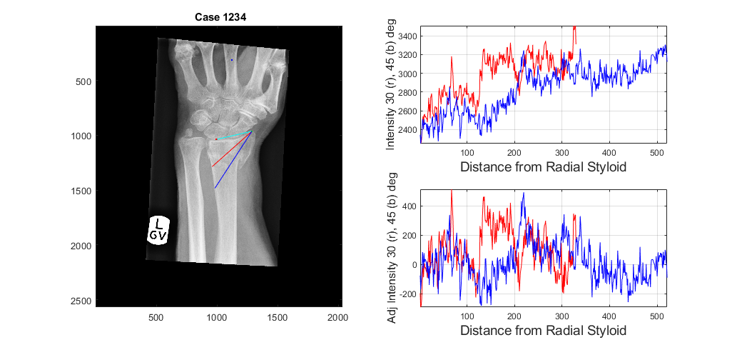
To determine two profiles from the radial styloid to the edge of the radius at 30 and 45 degrees below the line between the radial styloid and the lunate the function analyseLandmarkRadial is used in the following way:
displayData = 1;[stats,displayResultsRadial] = analyseLandmarkRadial (XrayR2,Xray_maskR,Xray_info,'Case 1234',displayData);
Notice that we have used the variable "displayData", which if set to 1, prompts the data to be displayed in a new figure. If it is set to 0 (or not passed as an input variable) no new figure is generated. In addition, the name of the case ('Case 1234') has been passed as an input.
The output variable 'stats' contain values about the lines (slope, standard deviation, etc)
stats
stats =struct with fields:
slope_1: 1.9149 slope_2: 1.5220 slope_short_1: 6.6215 slope_short_2: 3.8167 std_1: 243.0131 std_2: 252.0656 std_ad_1: 153.6793 std_ad_2: 131.0886 row_LBP: 1189 col_LBP: 1060
In addition displayResultsRadial contains the actual profiles of the lines, as well as the data with the profiles and the landmarks.
displayResultsRadial
displayResultsRadial =struct with fields:
prof_radial_new1: [329×1 double] prof_radial_new2: [521×1 double] prof2_radial_new1: [329×1 double] prof2_radial_new2: [521×1 double] dataOutput: [2567×2033×3 double] dist_prof_1: 44.6530 dist_prof_2: 58.4762
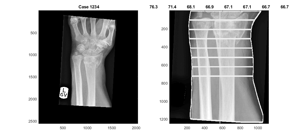
The landmark of the lunate is used to determine the forearm, and from there delineate the edges of the arm, and trace 8 lines that measure the width of the forearm, each at one cm of separation. The widths are displayed on the figure when you select to display.
[edgesArm,widthAtCM,displayResultsLunate,dataOutput,coordinatesArm] = analyseLandmarkLunate (XrayR2,Xray_maskR,Xray_info,'Case 1234',displayData);
Of the previous output variables, edgesArm is a 2D matrix with the delineation of the arm, displayResultsLunate is a 2D matrix with the lines overlaid on the original Xray, dataOutput is the same, except that the lines are in red for better contrast. widthAtCM are the actual width of each line. coordinatesArm are the rows and columns that are used to crop the forearm.
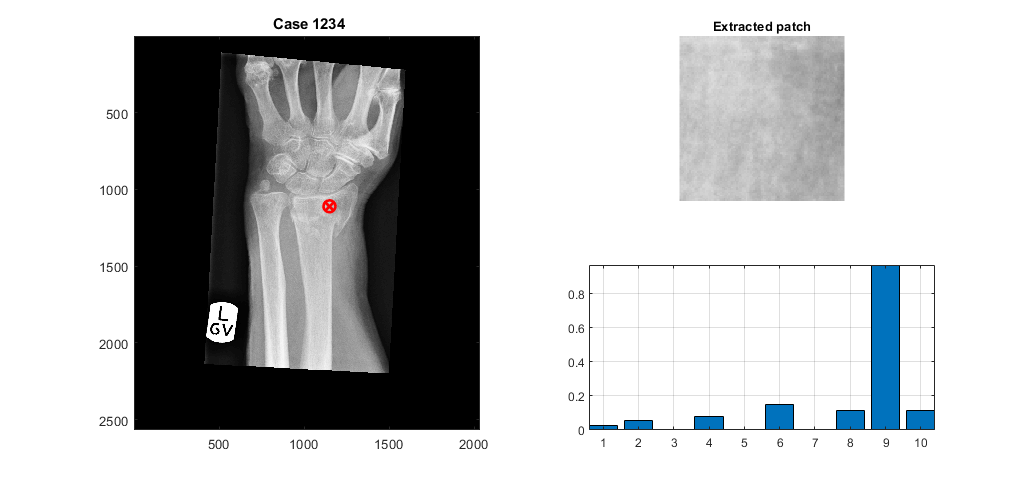
A region of interest is detected and the Local Binary Pattern is calculated, the location of the region is selected as an intermediate point of the previously located profiles, so these are necessary input parameters.
sizeInMM                        = [5, 5];
[LBP_Features,displayResultsLBP]    = ComputeLBPInPatch(XrayR2,Xray_info,Xray_maskR,stats.row_LBP,stats.col_LBP+50,sizeInMM,displayData);
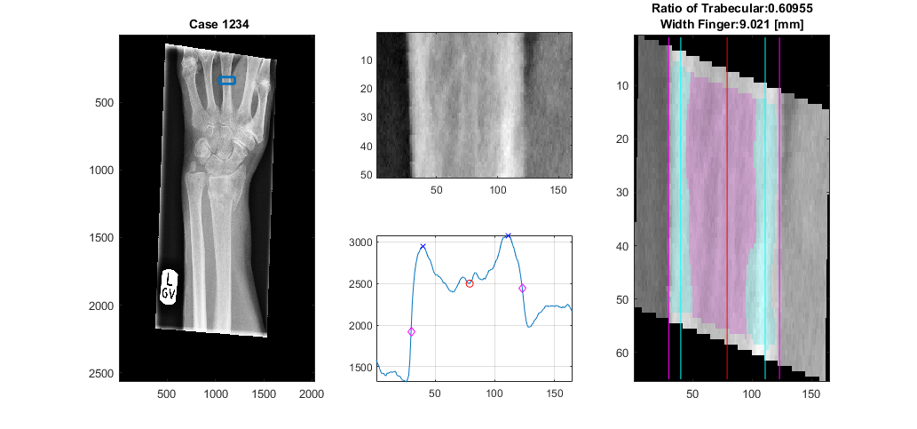
The analysis of the landmark of the central finger segments the bone according to the trabecular and cortical regions and then calculates the ratio.
[TrabecularToTotal,WidthFinger,displayResultsFinger] = analyseLandmarkFinger (XrayR,Xray_maskR,Xray_info,'Case 1234',displayData);
There are several ways to display and visualise the data. Try the files that start with displayXray*.m. For example to generate videos you can try:
[dataOut,dataOut2,displayResults] = extract_measurements_xray(currentFile,Xray,Xray_info,Xray_mask);
allHandles = displayXrayAnimation(displayResults,dataOut);
