README

Data Modeling with PostgreSQL

Model user activity data to create a database and ETL (Extract, Transform, Load) pipeline in PostgreSQL for a music streaming app and define a Fact and Dimension tables.

Table of Content

Introduction
Project Description
Project Development
Pipeline ETL
- Execution Instructions
- Troubleshooting
  - Create Tables
  - ETL Pipeline
Expected Results
Discussion

Introduction

A startup called Sparkify wants to analyze the data they have been collecting on songs and user activity on their new music streaming app. The analytics team is particularly interested in understanding what songs users are listening to. Currently, they do not have an easy way to query the data, which resides in a directory of JSON logs on user activity on the app, as well as a directory with JSON metadata on the songs in their app.

It is required to a PostgresSQL database with tables designed to optimize queries on song play analysis creating a database schema and ETL pipeline for this analysis.

The database and ETL process are requited to be tested by running given queries by the analytics team from Sparkify and comparing the outputs with the expected results.

Project Description

In the project is applied knowledge about data modeling with PostgreSQL and ETL pipeline using Python. Fact and Dimension tables are designed in a star schema for a particular analytic focus, and the ETL pipeline transfers data from files in two local directories into the mentioned tables in PostgreSQL using Python and SQL.

Project Development

To develop all the project, it is already defined the Schema, but no the complete database structure, also, the raw data is only available in JSON files, so a ETL pipeline is required, the following sections describe how the project is handled.

Datasets

To understand the requirements, business purposes and technical characteristics of the project the first step is get the datasets into the development environment.

Download the Datasets

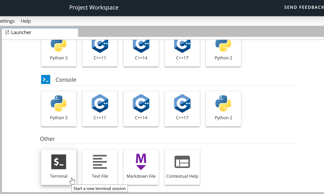
Access to Udacity's Project Workspace and open a Terminal.

Inside the terminal type the following command:
```
zip -r data.zip data
```
In the workspace directory (/home/workspace) a new file will appear and it is called data.zip, download the file.

On this case, the data.zip is also available in a personal drive to download the datasets.

Dataset Tree Directory

Locate the data directory in the root path of the development environment, all JSON files are located here, the following diagram shows the current directory tree.

<root_path>/data_modeling_postgresql_deu_01/data
├───log_data
│   └───2018
│       └───11
└───song_data
    └───A
        ├───A
        │   ├───A
        │   ├───B
        │   └───C
        └───B
            ├───A
            ├───B
            └───C

Song Dataset

Subset of real data from the Million Song Dataset. Each file is in JSON format and contains metadata about a song and the artist of that song. The files are partitioned by the first three letters of each song's track ID. Below are the root tree directory and filepath examples of two files in the dataset.

<root_path>/data_modeling_postgresql_deu_01/data/song_data
└───A
   ├───A
   │   ├───A
   │   ├───B
   │   └───C
   └───B
      ├───A
      ├───B
      └───C

<root_path>/data_modeling_postgresql_deu_01/data/song_data/A/A/B/TRAABCL128F4286650.json
<root_path>/data_modeling_postgresql_deu_01/data/song_data/A/B/C/TRABCYE128F934CE1D.json

Below is an example of what a single song file looks like (TRABCAJ12903CDFCC2.json):

{
  "num_songs": 1,
  "artist_id": "ARULZCI1241B9C8611",
  "artist_latitude": null,
  "artist_longitude": null,
  "artist_location": "",
  "artist_name": "Luna Orbit Project",
  "song_id": "SOSWKAV12AB018FC91",
  "title": "Midnight Star",
  "duration": 335.51628,
  "year": 0
}

It is important to identify what is the content of the available files, sometimes, the name of the attributes helps to know the type of data to store, for example, the duration attribute and current value indicates that is not possible to have sentences here, so at designing the database a good type of data could be float or numeric.

It is a recommendation to visualize more than one JSON file, it helps to understand data better and identify possible inconsistencies or common missing values.

Log Dataset

Consists of log files in JSON format generated by this event simulator based on the songs in the dataset songs. These simulate activity logs from a music streaming app based on specified configurations. Below are the root tree directory and filepath examples of two files in the dataset, the log files in the dataset are partitioned by year and month.

<root_path>/data_modeling_postgresql_deu_01/data/log_data
├───log_data
    └───2018
        └───11

<root_path>/data_modeling_postgresql_deu_01/data/log_data/2018/11/2018-11-12-events.json
<root_path>/data_modeling_postgresql_deu_01/data/log_data/2018/11/2018-11-13-events.json

To look at the JSON data within log_data files, create a pandas dataframe to read the data (code example below), after the code block example, there is an example of what the data in a log file (2018-11-12-events.json) looks like.

import json
import os
import pandas as pd

song_log_path = os.path.join(
    os.getcwd(), "data/log_data/2018/11/2018-11-01-events.json"
)
song_logs_df = pd.read_json(song_log_path, lines=True)
songs_logs_df.head()

As mentioned in the previous section, it is important to identify what are the content of the available files, the name of the attributes helps to know the type of data to store, for example, the page attribute and values indicates that is possible to have only specific values and no numbers, just strings, so at designing the database a good type of data could be varchar or text.

It is a recommendation to visualize more than one JSON file, it helps to understand data better and identify possible inconsistencies or common missing values.

Comments:
Use this JSON file format (video). resource to better understand the JSON files.
HINT: Use the value_counts method on log dataframes, this is a good option to identify attributes that store only specific values, e.g:
      df["attribute_n"].value_counts()

Entity Relational Diagram (ERD)

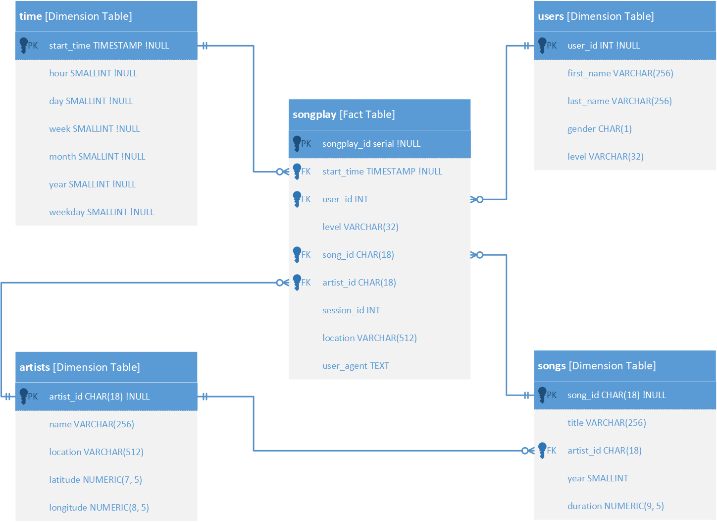
The Star Schema designed allows to create queries easily to retrieve specific business metrics; after seing some songs and logs JSON files, the following ERD resulted.

Comments:

During the development, some attributes changed, it is ok, it is not possible to check all the files, and sometimes some data structure is not identified until the development code process.

Local Database Setup

Make sure the PostgreSQL program is installed.
Open SQL Shell, use the Search tool and type psql.
Access under the following inputs:
1. Server: localhost
2. Database: postgres
3. Port: 5432
4. Username: postgres
5. Password: <Password_configured_at_installing_PostgreSQL>
Verify if the admin does not exists, if the role exists, go to step number X:
```
\du
```

Create the admin role:

CREATE ROLE admin WITH LOGIN ENCRYPTED PASSWORD '<password>';

Assign permissions to the created role:
```
ALTER ROLE admin CREATEDB;
```
Quit the SQL SHELL
```
\q
```
Open again the SQL Shell.
Access as admin, use the created
1. Server: localhost
2. Database: postgres
3. Port: 5432
4. Username: admin
5. Password: <Password_configured_at_creating_role_admin>

Create the database:

CREATE DATABASE data_modeling_postgres_01;

Quit SQL Shell.

Development Files

The development include the following scripts:

test.ipynb: Displays the first few rows of each table to check the database.
create_tables.py: Drops and creates the tables. Running this file resets the tables before each time to run the ETL scripts ( etl.ipynb and etl.py).
etl.ipynb: Reads and processes a single file from song_data and log_data, upload the data into the tables. This notebook contains instructions on the ETL process for each table.
etl.py: Reads and processes files from song_data and log_data and upload them into the tables. Based on the work in the ETL notebook (etl.ipynb).
sql_queries.py: Contains all the SQL queries, and it is imported by the last three files above.
requirements.txt> Contains the packages and versions used to run the project locally.

Inside each file there are the corresponding docstrings and execution description.

Setup Development Environment

The current project is developed in Anaconda installed on a Windows 10 OS; use the corresponding Python version (Python v.3.9.6 64-bit).

Check the Python version in the current environment using the following command line (it is assumed Miniconda or Anaconda is installed):

python --version
To verify the Python architecture installed use the following command:

python -c "import struct; print(struct.calcsize('P')*8)"

The number returned correspond to the architecture (32 for 32-bits and 64 for 64-bits).

It is important to have the same Python version to reduce incompatibilities when exporting the scripts from one environment to other, the following sections help to create a Python Virtual environment on case the Python version is not available in an existing virtual environment.

Create Environment

An environment helps to avoid packages conflicts, and it allows developing software under similar production conditions.

The environment is set using Anaconda Python package distribution.

Create a new environment:

conda create -n data_engineer python=3.9.6
Install pip into the new environment:

conda install -n data_engineer pip
After the environment creation, it is possible to activate it and deactivate it using the next commands:

conda activate data_engineer

conda deactivate

NOTES:

Get additional insights from the Anaconda Portal called Managing Environments.

There is a lot of information and useful tips online; use the Conda Cheat Sheet and this Towards Article to get additional insights about Anaconda environments.

WARNING!!!:

Install the management packages using conda and then use pip to install the development packages, it avoids unexpected behaviors, never try to use conda installer after using for the first time the command pip to install packages.

Create Jupyter Kernel Environment

Verify the Jupyter Notebook installation in the root environment:

conda install jupyter
Activate the development environment and install the Jupyter Kernel:

conda activate data_engineer

conda install ipykernel
Link the Jupyter Kernel to Jupyter Notebook:
python -m ipykernel install --user --name data_engineer --display-name "Python v.3.9.6 (data_engineer)"
Launch the Jupyter Notebook, and check the new environment is available as a Jupyter Kernel option.

NOTES:

Get more insights about Jupyter Kernel Environments in this Stack Overflow Post.

Package Requirements

The package requirements are registered in their corresponding requirements.txt file, this file is created manually alongside the development process and in the same installation order.

It helps to avoid installation errors and incompatibilities at setting environments on different machines.

The following command lines help to list correctly the package requirements and versionig.

List the installed packages and versions:

pip freeze

pip list --format=freeze
If the requirements.txt file is completed or it is required to replicate the environment using the current development, use the next command line to install again the packages due to an environment crashing:

pip install -r requirements.txt

If the installation does not run correctly, use the next command to install one-by-one the required packages and versions following the requirements.txt packages and versions:

pip install <package>==<version_number>

Pipeline ETL

Execution Instructions

Open a command prompt and activate the environment:

conda activate data_engineer
Into the current working directory (<root_path>/data_modeling_postgresql_deu_01/), execute the script to create the corresponding database tables:

python create_tables.py
Once the process finished, run the ETL pipeline:

python etl.py

The last script execution must shows a similar output as bellow.

Send 'time' records batch from idx '0'...
Send 'users' records batch from idx '0'...
Get 'song_id' and 'artist_id' on batch from idx '0'...
Send 'songplays' records batch from idx '0'...
30/30 files processed.

How many rows have song_id and artist_id in table 'songplay'?

Use the following SQL statement:
SELECT *
FROM songplay s
WHERE  s.song_id IS NOT NULL AND s.artist_id IS NOT NULL;

There are 1 rows with this data in 'songplay' table :c

songplay_id                start_time  user_id  level  ...    user_agent
          0  4627 2018-11-21 21:56:47       15   paid  ...  "Mozilla..."

[1 rows x 9 columns]

Troubleshooting

Create Tables

At the execution of create_tables.py shows an error similar to below.

ERROR: Connection to the PostgreSQL database failed!!! :c
FATAL:  password authentication failed for user "admin"

Complete log error:
Traceback (most recent call last):
File "<root>\data_modeling_postgresql_deu_01\create_tables.py", line <X>, in create_database
   conn = psycopg2.connect(
File "<root>\Miniconda3\envs\data_engineer\lib\site-packages\psycopg2\__init__.py", line <X>, in connect
   conn = _connect(dsn, connection_factory=connection_factory, **kwasync)
psycopg2.OperationalError: FATAL:  password authentication failed for user "admin"

To solve this error just verify the database credentials and change them to accomplish to the current environment, the following snip code shows where to change the credential inside the script create_tables.py, if the snip code no matches, just follows the parameters patterns user, passwrod, host, port and dbname to update the credentials.

 # Connect to 'sparkifydb' database
 try:
     conn = psycopg2.connect(
         user="admin",
         password="<password>",
         host="localhost", 
         port="5432",
         dbname="sparkifydb"
     )
     cur = conn.cursor()

 except psycopg2.Error as e:
     message = traceback.format_exc()
     print("ERROR: Connection to the PostgreSQL database failed!!! :c\n")
     print(f"Error:\n{e}\n")
     print(f"Complete log error:\n{message}\n")

 return cur, conn

# Connection to admin local database
 try:
     conn = psycopg2.connect(
         user="admin",
         password="<password>",
         host="localhost", 
         port="5432",
         dbname="data_modeling_postgres_01"
     )
     conn.set_session(autocommit=True)
     cur = conn.cursor()

ETL Pipeline

At the execution of etl.py shows an error similar to below.

Traceback (most recent call last):
File "<root>\data_modeling_postgresql_deu_01\etl.py", line <X>, in <module>
   main()
File "<root>\Data_Modeling_With_PostgreSQL\etl.py", line <X>, in main
   conn = psycopg2.connect(
File "<path>\Miniconda3\envs\data_engineer\lib\site-packages\psycopg2\__init__.py", line <x>, in connect
   conn = _connect(dsn, connection_factory=connection_factory, **kwasync)
psycopg2.OperationalError: FATAL:  password authentication failed for user "admin"

To solve this error just verify the database credentials and change them to accomplish to the current environment, the following snip code shows where to change the credentials inside the script etl.py, if the snip code no matches, just follows the parameters patterns user, passwrod, host, port and dbname to update the credentials.

 # Connect to 'sparkifydb' database
def main():
   conn = psycopg2.connect(
      user="admin",
      password="<password>",
      host="localhost",
      port="5432",
      dbname="sparkifydb"
   )
   cur = conn.cursor()

Expected Results

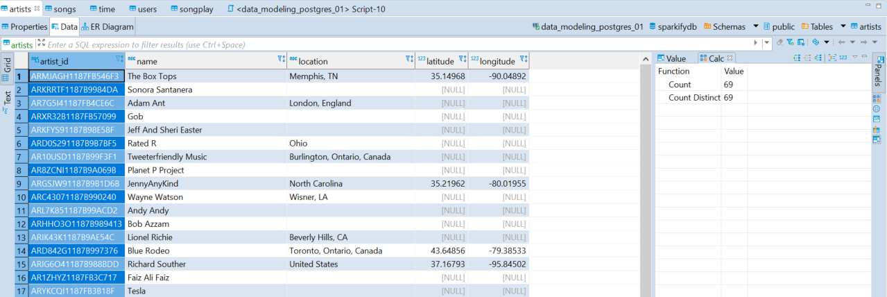
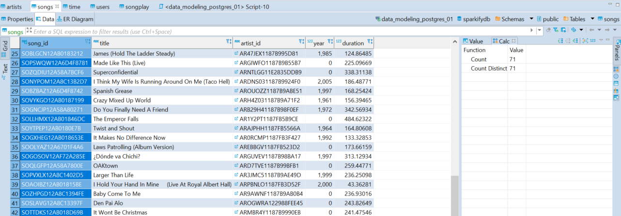
The following images shows the final tables content after executing the finished etl.py script, the images are extracted from the DBeaver Universal Database Manager v.7.2.5.202011152110

Artists Table

This table has 69 rows of artists data.

Songs Table

This table has 71 rows of songs data.

Users Table

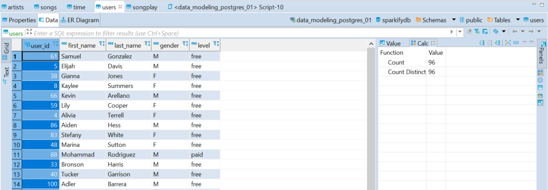
This table has 96 rows of users data.

Time Table

This table has 6813 rows of records of time.

Songplays Table

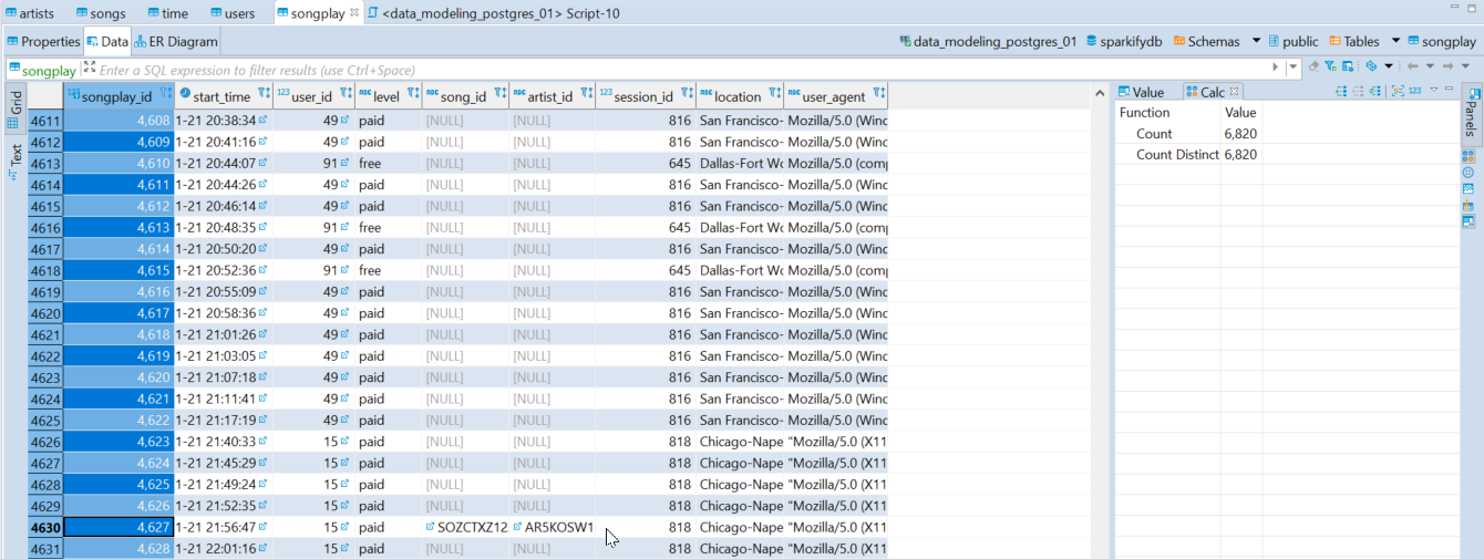
This table has 6820 rows of records of songplays.

As a detail noted, the table has only one row with complete data, to see the content just execute the following SQL statement on DBeaver or inside the test.ipynb.

Use this command in DBeaver:

SELECT *
FROM songplay s
WHERE  s.song_id IS NOT NULL AND s.artist_id IS NOT NULL;

Use this command in the Jupyter Notebook test.ipynb:

%sql %sql SELECT * FROM songplay s WHERE  s.song_id IS NOT NULL AND s.artist_id IS NOT NULL;

A similar table as below will show.

Discussion

The current database schema is focused on how frequent the users use the platform and identify which songs and artist are frequently heard.

Based on the sparkify database, it is possible to retrieve different metrics, some of them are:

How many users pays for the platform use?

%SELECT u."level", COUNT(u."level")
FROM users u
GROUP BY u."level";

level	count
free	74
paid	22

The intention is users paid for the use of the platform, and the metrics shows that less than 25% of users pay, comparing the number of paid licenses per month could indicates if a marketing campaign is working or not.

What are the most frequent hours the users use the platform?

SELECT t."hour", COUNT(t."hour") AS frequency
FROM songplay sp
JOIN "time" t
ON sp.start_time = t.start_time
GROUP BY t."hour"
ORDER BY frequency DESC
LIMIT 5;

Query result:

hour	frequency
16	542
18	498
17	494
15	477
14	432

This could help to decide at which hours put some marketing or promotions to free users.

About ETL pipeline

The ETL pipeline could have some issues, for example, as seeing in the image results, there a lot of missing artists and songs IDs, at this point it is required to speak with Sparkify's responsibles, because it is important to know how to assing those IDs, using an arbitrary ID? waiting until new songs data files appears?

rgonzalezc1811/data_modeling_postgresql_deu_01