A workshop on understanding and using projections for spatial data in R
The expected outcome of this workshop is not that you will understand everything about projections by the end of the 2 hours. Learning and understanding projections for geospatial data is (perhaps unfortunately) a life-long endevor. My expectation is that by the end of this workshop, you will have a better understanding of what a projection is, why you would choose one over another, and how to apply them correctly to geospatial data in R. Will you have questions later? Of course! That is entirely expected.
Learning is sometimes difficult. Projections are confusing. As I stated early, I hope to mitigate this, but let's recognize it up front. I have some rules for my classroom for just these kinds of situations:
- I expect you to ask questions.
- I want you to ask "dumb" questions as well as "smart" questions (whatever those terms mean for you). All questions are valid.
- You may answer questions. I highly encourage you to discuss your questions with others in the room. Maybe you can figure it out together. If you want more input, ask someone else.
- I will do my best to answer your questions, but reserve the right to say "I don't know" or "I will need to do some research and get back to you" or ask the people in the room if they know the answer. One person can't know everything.
- You can and should take breaks when you need to. Step outside, walk around, I won't be offended. Brains need a break. If you need to take this home and work on it later, that's fine too!
CRS = Datum + Projection + Additional Parameters
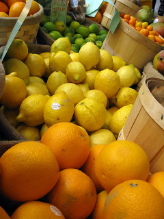
A common analogy employed to teach projections is the orange peel analogy. If you imagine that the earth is an orange, how you peel it and then flatten the peel is similar to how projections get made. We will also use it here.
A Datum is a model of the shape of the earth.
It has angular units (i.e. degrees) and defines the starting point (i.e. where is (0,0)?) so the angles reference a meaningful spot on the earth.
Common global datums are WGS84 and NAD83. Datums can also be local, fit to a particular area of the globe, but ill-fitting outside the area of intended use.
When datums are used by themselves it's called a Geographic Coordinate System.
Orange Peel Analogy: a datum is your choice of fruit to use in the orange peel analogy. Is the earth an orange, a lemon, a lime, a grapefruit?
Comments from the pros: Datums matter! California Albers with NAD27 is NOT the same as California Albers with NAD83. See all of the advice here
A Projection is a mathematical transformation of the angular measurements on a round earth to a flat surface (i.e. paper or a computer screen).
The units associated with a given projection are usually linear (feet, meters, etc.).
Many people use the term "projection" when they actually mean "coordinate reference system". (With good reason, right? Coordinate References System is long and might make you sound pretentious.) One example is the title of this workshop... but you wouldn't know what it was about if I said it was a workshop on "Coordinate Reference Systems in R", would you?
Orange Peel Analogy: a projeciton is how you peel your orange and then flatten the peel.

Image source: http://blogs.lincoln.ac.nz/gis/2017/03/29/where-on-earth-are-we/
Additional parameters are often necessary to create the full coordinate reference system. For example, one common additional parameter is a definition of the center of the map. The number of required additional parameters depends on what is needed by each specific projection.
Orange Peel Analogy: an additional parameter could include a definition of the location of the stem of the fruit.
To decide if a projection is right for your data, answer these questions:
- What is the area of minimal distortion?
- What aspect of the data does it preserve?
University of Colorado's Map Projections and the Department of Geo-Information Processing has a good discussion of these aspects of projections. Online tools like Projection Wizard can also help you discover projections that might be a good fit for your data.
Comments from the pros: Take the time to figure identify a projection that is suited for your project. You don't have to stick to the ones that are popular.
You have two options for identifying a CRS in most R commands. The documentation for a command that requires projection information will tell you which is required. Often you can choose between the two options.
A note on linguistics: EPSG stands for "European Petroleum Survey Group"... but everyone just says EPSG.
An EPSG Code is an ID that has been assigned to most common projections to make reference to a particular projection easy. An EPSG Code is also called an SRID (Spatial Reference Identifier). Technically, EPSG is the authority that assigns SRIDs, but you will hear these terms used interchangibly.
The main advantages to using this method of specifying a projection are that it is standardized and ensures you have the same parameters every time. The disadvantage is that if you need to know the parameters used by the projection or it's name, you have to look them up, but that's fairly easy to to at spatialreference.org. Also, you can't customize the parameters if you use an EPSG code. For example: EPSG:27561
PROJ.4 is an open source library for defining and converting between coordinate reference systems. It defines a standard way to write projection parameters. For example: +proj=lcc +lat_1=49.5 +lat_0=49.5 +lon_0=0 +k_0=0.999877341 +x_0=6 +y_0=2 +a=6378249.2 +b=6356515 +towgs84=-168,-60,320,0,0,0,0 +pm=paris +units=m +no_defs
Two important advantages to using this option are (1) the parameters are human-readable and immediately transparent and (2) the strings are easily customized. The main disadvantage to this option is that it's easy to make a mistake when you reproduce the string, accidentally changing parameters.
A note on linguistics: PROJ.4 is commonly pronounced "prodge four" ("PROJ" rhymes with "dodge"); PROJ is short for "projection". The 4 is because we're currently using the 4th version of this library.
The #1 biggest mistake I see in any GIS (ArcMap, QGIS, R, GRASS, Python, etc.) is defining a projection for a dataset when the person should have re-projected the data. It is very common that you'll need to tell your GIS what the projection/CRS of your data should be. In these cases, the GIS needs to know what the projection/CRS currently is, not what you would like it to be. If you need to change a projection, you need to go through a different process, often called Re-project or Transform.
Finally, now we're going to work in R to get some hands-on practice with the concepts we just discussed.
We'll be working with sp objects today, but you should also know that there are sf objects as well. Roger Bivand's review of spatial data for R is helpful for understading the options for working with spatial data.
The data for this workshop is available in the data folder in this repository, or you can download a .zip file from FigShare.
Pick the R flavor of your choice - regular R, R Studio, etc. - and start it up. You can either add the commands we'll be using to a script file to run, or you can just run the lines individually in your console to see how they work. It's up to you.
TIP: I add to this section as I write my code and need new libraries. Keep them in one place for easy reference.
library(raster)
library(geojsonio)
library(rgdal)
TIP: Windows users, use \\ instead of \ or switch the direction of the slashes to /... it has to do with escape characters.
setwd("C:\\Workshops\\Data")
Replace C:\Workshops\Data with the path to the folder in which you saved your data.
Because "points" by itself is a command so we don't want confusion, I've added "ws." (WS for watershed) to the front of my variables.
Our data is in geojson format so we need a command that reads that format. Use the command ?geojson_read in your console to see the documentation for the geojson_read function.
ws.points<-geojson_read("WBDHU8_Points_SF.geojson", what="sp")
ws.polygons<-geojson_read("WBDHU8_SF.geojson", what="sp")
The streams data is a shapefile, so we'll load it with a different command than we used for our points and polygons. The Raster package has commands to read in other file types like rasters but also vectors like shapefiles.
ws.streams<-shapefile("flowlines.shp")
Let's look at one of the files:
ws.polygons
Note that the "coord. ref." (coordinate reference system... CRS) string is a PROJ.4 string. "+proj=aea +lat_1=34 +lat_2=40.5 +lat_0=0 +lon_0=-120 +x_0=0 +y_0=-4000000 +ellps=GRS80 +towgs84=0,0,0,0,0,0,0 +units=m +no_defs "
To see just the coordinate reference system, we can use the crs() command. Let's check the CRS for each of our files:
crs(ws.points)
crs(ws.polygons)
crs(ws.streams)
It looks like the streams dataset is missing a CRS.
Let's be clear that the streams data has a CRS, but the computer doesn't know what it should be. (Someone may have forgotten to include the .prj file in this shapefile.) You don't get to decide what you want it to be, but rather figure out what it should be and tell the computer what it should use. How? Typically, you first ask the person who sent it. If that fails, you can search for another version of the data online to get a file with the correct projection information. Finally, outright guessing can work, but isn't recommended. We know that the CRS for this data should be EPSG 3309 (because that's what the instructor saved it as before she deleted the .prj file... shapefiles are not a great exchange format, FYI).
Set the CRS:
crs(ws.streams)<-"+proj=aea +lat_1=34 +lat_2=40.5 +lat_0=0 +lon_0=-120 +x_0=0 +y_0=-4000000 +datum=NAD27+units=m +no_defs +ellps=clrk66 +nadgrids=@conus,@alaska,@ntv2_0.gsb,@ntv1_can.dat"

# or

crs(ws.streams)<-CRS("+init=epsg:3309")
Let's imagine we loaded up our data and find that it shows up on a map in the wrong location. What happened? Someone defined the CRS incorrectly. How do you fix it? First you figure out what the CRS should be, then you run one of the lines above with the correct CRS definition to fix the file.
We need to get all our data into the same projection so it will plot together on one map before we can do any kind of spatial process on the data.
Assign the PROJ.4 string from the other files to a variable:
newcrs<-crs(ws.polygons)
use the variable containing the CRS we want to use with the PROJ.4 string in spTranform()
ws.streams<-spTransform(ws.streams, newcrs)
Let's check the CRS for each of our files again:
crs(ws.points)
crs(ws.polygons)
crs(ws.streams)
Now they all should match.
Lets make a map now that all our data is in the same projection. What if we had tried to do this earlier before we fixed out projection definitions and transformed the files into the same projections?
Load up the CA Counties layer to use as reference in a map:
ca.counties<-geojson_read("CA_Counties.geojson", what="sp")
Let's plot all the data together:
plot(ca.counties, col="#FFFDEA", border="gray", xlim=bbox(ws.polygons)[1:2], ylim=bbox(ws.polygons)[3:4], bg="#dff9fd",  main = "Perennial Streams in the San Francisco Bay Watersheds")
plot(ws.streams, col="#3182bd", lwd=1.75, add=TRUE)
plot(ws.points, col="black", pch=20, cex=3, add=TRUE)
plot(ws.polygons, lwd=2, border="grey35", add=TRUE)
Some explanation of the code above for plotting the spatial data:
xlim/ylimsets the extent. Here I used the numbers from the bounding box of the polygon dataset, but you could put in numbers - remember that this is projected data so lat/long won't workadd=TRUEmakes the 2nd, 3rd, 4th, etc. datasets plot on the same map as the first dataset you plot - order matterscolsets the fill color for the geometrybordersets the outline color (or stroke for users of vector graphics programs)bgsets the background color for the plot- colors can be specified with words like "gray" or html hex codes like #dff9fd
After completing this workshop, you should now have a better understanding of Coordinate Reference Systems (CRS) or projections, as they are often called colloquially. You can now find out what the CRS is for a dataset and know the common formats this can take. You should understand the difference between defining a CRS and tranforming a dataset (often called "reprojecting" in other GIS programs), when to use them, and how to execute both commands. You've also seen how to use the basic plot() function to make a map.
Now that you've had some hands-on experience with projections and spatial data, it's a good time to go back an review the concepts introduced in the beginning of the workshop. You may find that some of it makes more sense now that you have more experience.
Do you now feel like you know everything you need to know and will never have any more questions? Of course not! It's a learning process that will continue for the rest of your career working with spatial data. Need more help? See data.ucdavis.edu for how to contact your friendly UC Davis GIS Data Curator.
- Rspatial.org
- Data Carpentry Intro to Geospatial Data with R
- University of Colorado's Map Projections
- International Institute for Geo-Information Science and Earth Observation (ITC)
- Carlos Furuti's Projections Page
Map Projection Fun:
- xkcd's Map Projections
- Jason Davies' Map Projection Transitions
- Carlos Furuti's Printable Projections Global projections you can print and assemble