DiscretePDEs.jl is a package for discretizing partial differential equations using DiscreteExteriorCalculus.jl. 3D visualization and meshing is performed with Gmsh. Geometrical models can be created using the Gmsh scripting functionality or by importing a GDS file. LayoutEditor is a convenient program for creating and manipulating GDS files.
In addition to functionality for discretizing arbitrary PDEs, DiscretePDEs.jl also has functionality specifically for modeling electromagnetism:
- Electrostatic fields and the capacitance matrix.
- Magnetostatic fields and the inductance matrix, including the London equation.
- Electrodynamic Positive Second Order models
including Ohm's Law and the London equation, using AdmittanceModels.jl
- Normal modes.
- Transfer functions.
The tests in the test folder also serve as in-depth examples for each of these problem
types.
Clone the repository from GitHub and install Julia 1.1. Then use the Julia package manager to activate and build. Since the build can take a while, you may prefer using Pkg; Pkg.build(verbose=true).
Notes on build: This package has two non-Julia dependencies. One is Gmsh, a 3D visualization and meshing program, and the other is gdspy, a Python package for manipulating GDS files. The deps/build.jl file configures the gmsh and gdspy dependencies and installs them if they are not present.
For gmsh
- If
ENV["gmshjl"]is set orgmshjl=...is in adeps/.envfile, thegmsh.jlfile at the indicated path is used. Precedent is given to the environment variable over thedeps/.enventry. - Else if a
gmsh.jlfile can be found somewhere within/usr/bin, thatgmsh.jlfile is used. - Else
gmsh.jlis installed usingdeps/install_gmsh.sh. This will work on Mac OSX or Linux Ubuntu:18.10.
For gdspy
- If
ENV["PYTHON"]is set orPYTHON=...is in thedeps/.envfile, thepythonbinary at the indicated path is used. Precedent is given to the environment variable over the.enventry. - Else
- If
which condafails, andminiconda3is not already present in the home directory,miniconda3is installed in the home directory. The.bashrcand.bash_profileetc. are not modified. - If a
DiscretePDEscondaenvironment does not already exist, one is made using thedeps/conda_env.ymlfile. Thepythonfrom thiscondaenvironment is used to buildPyCall.jl.
- If
If this all succeeds, the paths to gmsh.jl and python are saved in deps/.env so later builds will use the same gmsh and python.
See test/test_modes_box.jl for a more complete version of this example.
Import packages.
using DiscreteExteriorCalculus, DiscretePDEs
using AdmittanceModels: lossless_modes_dense, apply_transform
using LinearAlgebra: norm
Create a file box.geo that describes a 10×12×14 box.
a, b, c = 10, 12, 14
file_name = joinpath(@__DIR__, "box.geo")
geo_write!(file_name, characteristic_length_factor=1,
    footer="""
    Box(1) = {0, 0, 0, $a, $b, $c};
    """)
Start gmsh, open the file, mesh the box, and create a TriangulatedComplex for the primal
mesh.
initialize!()
gmsh_open!(file_name)
N, K = 3, 4
mesh!(K)
node_tags, points, tcomp = get_triangulated_complex(N, K)
Orient the primal mesh, compute the dual mesh, and put them both into a Mesh object.
orient!(tcomp.complex)
m = Metric(N)
mesh = Mesh(tcomp, circumcenter(m))
Create a Positive Second Order model and apply the Coulomb gauge and boundary condition constraints.
comp = tcomp.complex
μ⁻_form = get_material(comp, 1/DiscretePDEs.μ₀, 3)
Λ⁻_form = get_material(comp, 0, 2)
σ_form = get_material(comp, 0, 2)
ϵ_form = get_material(comp, DiscretePDEs.ϵ₀, 2)
pso, null_basis = electrodynamics_pso(m, mesh, Vector{Cell{N}}[], boundary(comp),
    μ⁻_form, Λ⁻_form, σ_form, ϵ_form)
constrained_pso = apply_transform(pso, null_basis)
Find the normal modes of the box.
λs, vs = lossless_modes_dense(constrained_pso)
freqs = imag(λs)/(2π)
Plot the mesh and lowest normal mode using gmsh.
vec_A = sharp(m, comp, null_basis * vs[:,1])
vec_A /= maximum(norm.(vec_A))
comp_points = [c.points[1] for c in comp.cells[1]]
ordering = [findfirst(isequal(p), comp_points) for p in points]
add_field!("Vector potential", node_tags, vec_A[ordering])
gui!()
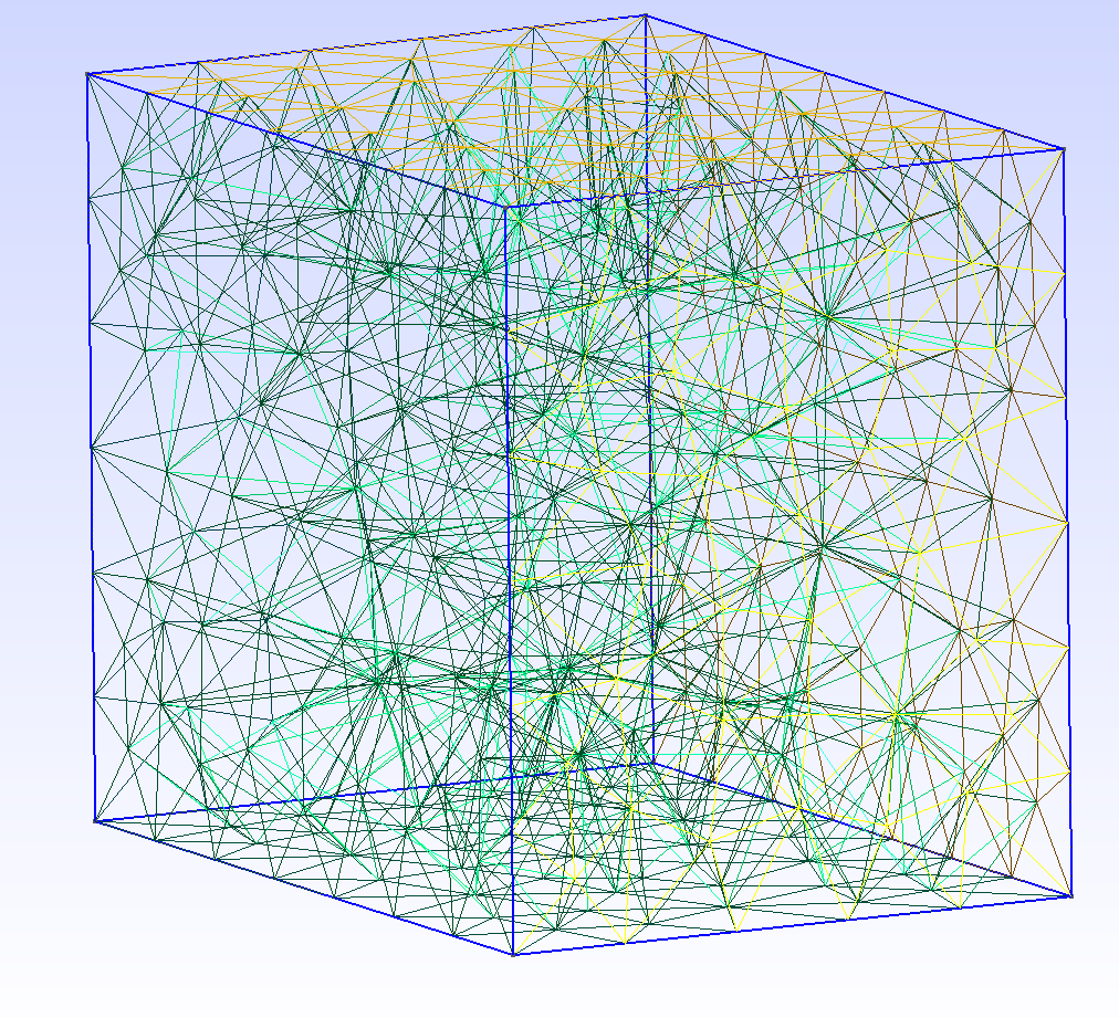
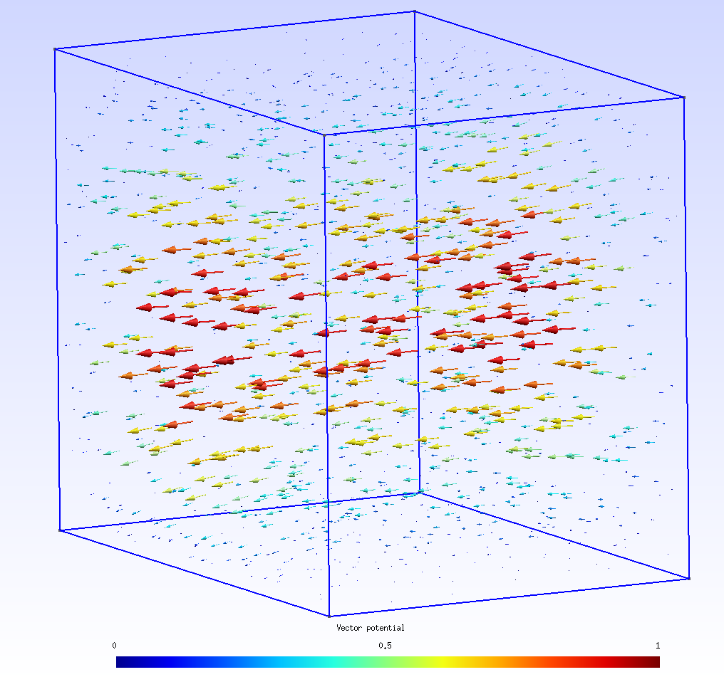
Mesh:  Lowest normal mode vector potential:
See test/test_cpw_resonator.jl. A non-uniform mesh with 7282 tetrahedra is used.
Mesh:  Lowest normal mode vector potential:
  Second lowest normal mode vector potential: