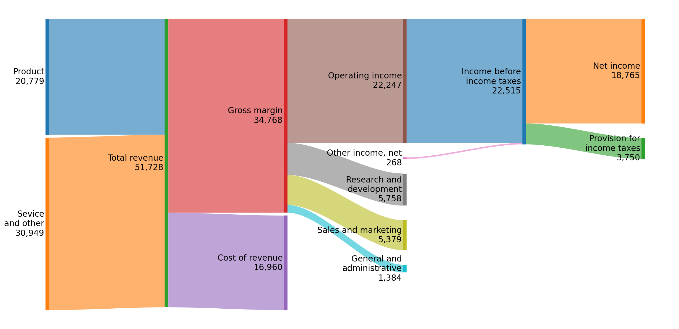
SankeyFlow

SankeyFlow is a lightweight python package that plots Sankey flow diagrams using Matplotlib.

import matplotlib.pyplot as plt
from sankeyflow import Sankey

flows = [
    ('Product', 'Total revenue', 20779),
    ('Sevice and other', 'Total revenue', 30949),
    ('Total revenue', 'Gross margin', 34768),
    ('Total revenue', 'Cost of revenue', 16960),
    ...
]
s = Sankey(flows=flows)
s.draw()
plt.show()

See example/msft_FY22q2.py for full example.

Description

While Matplotlib does have a builtin sankey class, it is designed around single node flows. SankeyFlow instead focuses on directional flows, and looks more similar to plotly and SankeyMATIC. It also treats nodes and flows separately, so the node value, inflows, and outflows don't have to be equal.

SankeyFlow is also fully transparent with Matplotlib; the sankey diagram requires only an axis to be drawn: Sankey.draw(ax). All elements in the diagram are Matplotlib primitives (Patch and Text), and can be directly modified with the full suite of Matplotlib options.

Installation

Requires Matplotlib and numpy.

python3 -m pip install sankeyflow

You can then simpliy

from sankeyflow import Sankey

Usage

The core class is sankeyflow.Sankey, which builds and draws the diagram. Data is passed in the constructor or with Sankey.sankey(flows, nodes), and the diagram is drawn with Sankey.draw(ax).

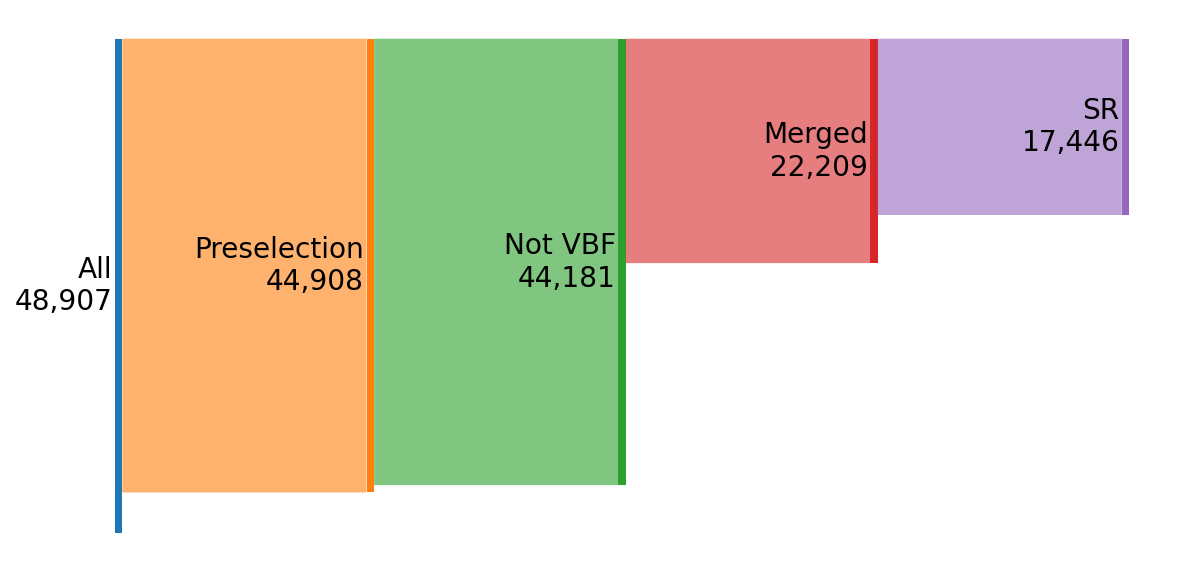
The diagram defaults to a left-to-right flow pattern, and breaks the nodes into "levels," which correspond to the x position. The cutflow diagram above has 5 levels, for example.

nodes is a nested list of length nlevels, ordered from left to right. For each level, there is a list of nodes ordered from top to bottom. Each node is a (name, value) pair.
flows is a list of flows, coded as (source, destination, value). source and destination should match the names in nodes. Additionally, if value is given as a tuple, the value can represent the start and end value of the flow, respectively.

If nodes is None, the nodes will be automatically inferred and placed from the flows.

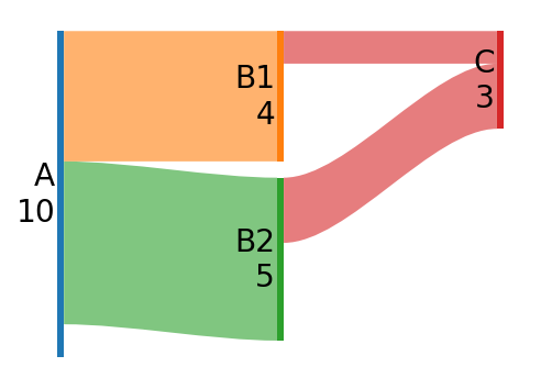
nodes = [
    [('A', 10)],
    [('B1', 4), ('B2', 5)],
    [('C', 3)]
]
flows = [
    ('A', 'B1', 4),
    ('A', 'B2', 5),
    ('B1', 'C', 1),
    ('B2', 'C', 2),
] 

plt.figure(figsize=(4, 3), dpi=144)
s = Sankey(flows=flows, nodes=nodes)
s.draw()

Configuration

Diagram and global configuration are set in the constructor. Individual nodes and flows can be further modified by adding a dictionary containing configuration arguments to the input tuples in Sankey.sankey(). See docstrings for complete argument lists.

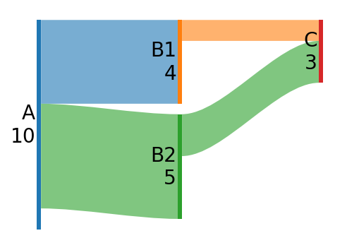
For example, we can change the colormap to pastel, make all flows not curvy, and change the color of one flow.

flows = [
    ('A', 'B1', 4),
    ('A', 'B2', 5),
    ('B1', 'C', 1),
    ('B2', 'C', 2, {'color': 'red'}),
] 

s = Sankey(
    flows=flows,
    nodes=nodes,
    cmap=plt.cm.Pastel1,
    flow_opts=dict(curvature=0),
)
s.draw()

By default the color of the flows is the color of the destination node. This can be altered globally or per-flow with flow_color_mode.

flows = [
    ('A', 'B1', 4),
    ('A', 'B2', 5, {'flow_color_mode': 'dest'}),
    ('B1', 'C', 1),
    ('B2', 'C', 2),
] 

s = Sankey(
    flows=flows,
    nodes=nodes,
    flow_color_mode='source',
)
s.draw()

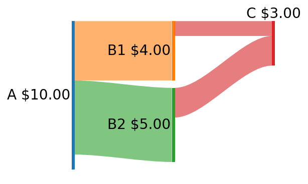
We can also easily adjust the label formatting and other node properties in the same way.

nodes = [
    [('A', 10)],
    [('B1', 4), ('B2', 5)],
    [('C', 3, {'label_pos':'top'})]
]
flows = [
    ('A', 'B1', 4),
    ('A', 'B2', 5),
    ('B1', 'C', 1),
    ('B2', 'C', 2),
] 

s = Sankey(
    flows=flows,
    nodes=nodes,
    node_opts=dict(label_format='{label} ${value:.2f}'),
)
s.draw()

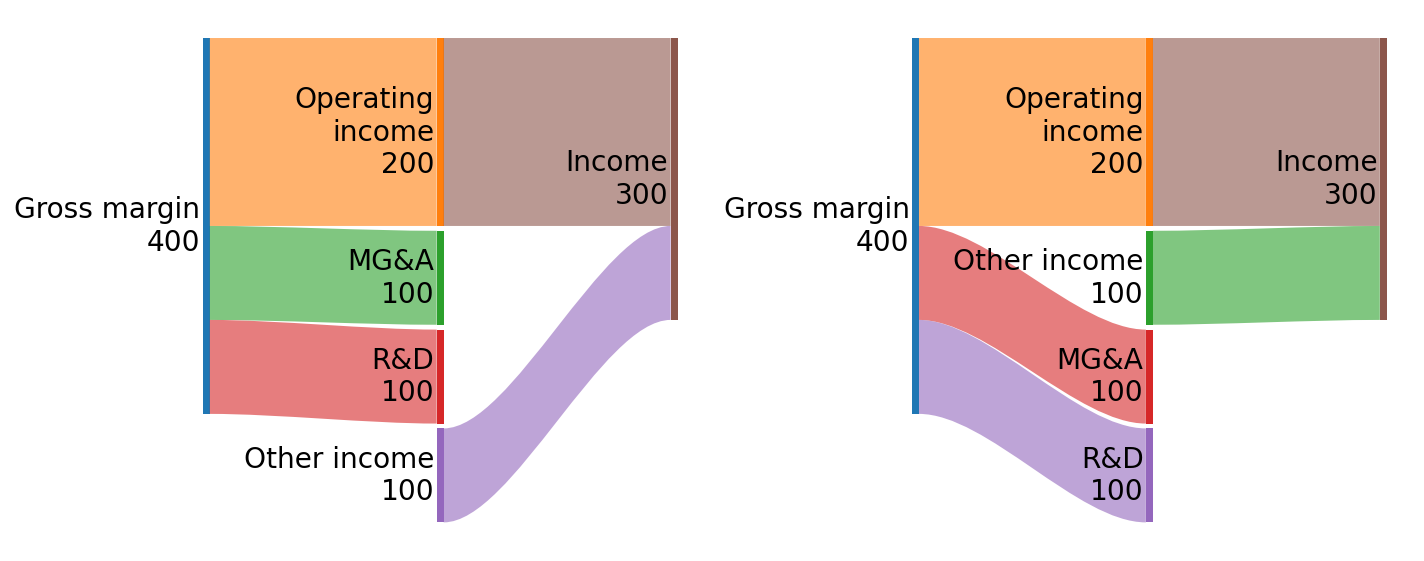
Automatic Node Inference

Nodes can be automatically inferred from the flows by setting nodes=None in Sankey.sankey(). They are placed in the order they appear in the flows.

gross = [
    ('Gross margin', 'Operating\nincome', 200),
    ('Gross margin', 'MG&A', 100), 
    ('Gross margin', 'R&D', 100), 
]
income = [
    ('Operating\nincome', 'Income', 200),
    ('Other income', 'Income', 100, {'flow_color_mode': 'source'}),
]

plt.subplot(121)
s1 = Sankey(flows=gross + income)
s1.draw()

plt.subplot(122)
s2 = Sankey(flows=gross[:1] + income + gross[1:])
s2.draw()

plt.tight_layout()

If you want to configure individual nodes while using the automatic inference, you can either access the nodes directly:

s = Sankey(flows=flows)
s.find_node('name')[0].label = 'My label'

or retrieve the inferred nodes and edit the list before passing to Sankey.sankey():

nodes = Sankey.infer_nodes(flows)
# edit nodes
s.sankey(flows, nodes)

The latter is the only way to edit the ordering or level of the inferred nodes.