Analysis code to generate figures and artifacts presented in Chapman, et al., “Risk-sensitive safety analysis using Conditional Value-at-Risk,” submitted to IEEE Transactions on Automatic Control, January 2021.
Running the code in this repository requires a recent version of Matlab. We have tested this repository using Matlab 2019b on Windows 10 and Red Hat Enterprise Linux Server release 7.8.
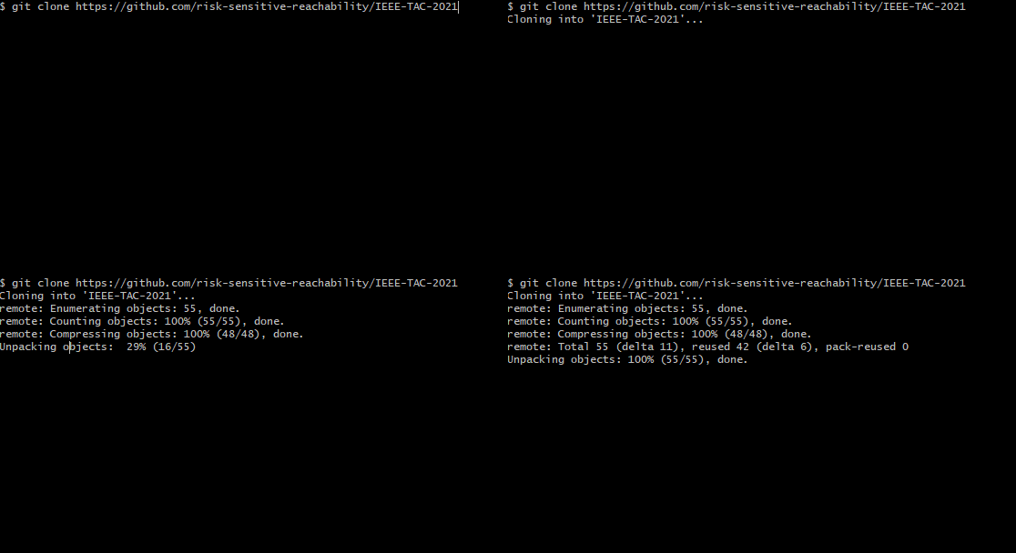
Using git is the easiest way to download a copy of all the files you need to get up and running in Matlab. We tested these instructions against git v2.8.2.396.
The files will be downloaded to a folder named IEEE-TAC-2021.
From a command line interface, navigate to the directory where you would like to download IEEE-TAC-2021.
Then execute the following command:
git clone https://github.com/risk-sensitive-reachability/IEEE-TAC-2021
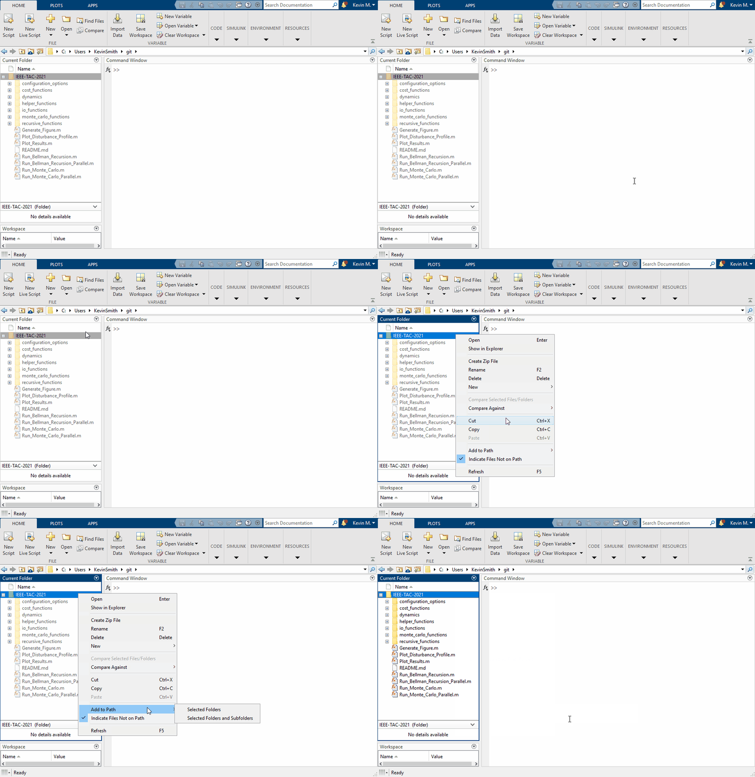
To setup your Matlab workspace:
- navigate to the parent directory containing IEEE-TAC-2021
- from the left-hand file tree, right click on IEEE-TAC-2021 and select Add To Path > Selected Folders and Subfolders.
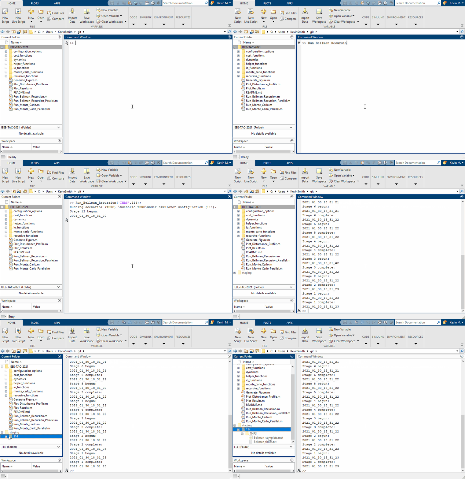
The first step in the analysis of a particular configuration and scenario combination is to call Run_Bellman_Recursion. The first argument is a string identifying the scenario to run and the second argument is an integer identifying the simulator configuration to use. See the computational prerequisites column in the list of figures at the bottom of this page for examples. Note that running this will create files in the {Matlab_Working_Directory}/staging/ directory. These include both 'checkpoint' files that save results periodically and 'complete' files that are created once the entire recursion is finished. Once you have obtained a 'Bellman_complete.mat' file you may run the Monte Carlo analysis. Note: this process can take several days to complete. If you have a parallel pool available, Run_Bellman_Recursion_Parallel is a parallel implementation that can speed up the process significantly.
The second step in the analysis of a particular configuration and scenario combination is to call Run_Monte_Carlo. This assumes you have already called Run_Bellman_Recursion and that process completed by producing a 'Bellman_complete.mat' file. The first argument to Run_Monte_Carlo is a string identifying the scenario to run and the second argument is an integer identifying the simulator configuration to use. See the computational prerequisites column in the list of figures at the bottom of this page for examples. Note that running this will create files in the {Matlab_Working_Directory}/staging/ directory. These include both 'checkpoint' files that save results periodically and 'complete' files that are created once the entire Monte Carlo analysis is finished. Once you have obtained a 'Monte_Carlo_complete.mat' you may move on to visualizing the results. Note: this process can take several days to complete. If you have a parallel pool available, Run_Monte_Carlo_Parallel is a parallel implementation that can speed up the process significantly.
The final step in the analysis of a particular configuration and scenario combination is to call the various plotting functions. This assumes you have already called Run_Monte_Carlo and that process completed by producing a 'Monte_Carlo_complete.mat' file for each scenario and configuration of interest. The first argument to Plot_Results is a string identifying the scenario and the second argument is an integer identifying the simulator configuration to use. The Plot_Disturbance_Profile method takes only a single string argument identifying the scenario. Generate_Figure is a convenience function for generating the Figures 3-8 shown in this paper and takes the Figure number as a single numeric argument (e.g., Generate_Figure(3)).
The first argument to Plot_Results is a string identifying the scenario and the second argument is an integer identifying the simulator configuration to use. This method will create plots relevent to the scenario of interest. For the 1-dimensional thermostatically controlled load examples (e.g., Plot_Results('THLS',114)) it produces two figures: (1) a grid of estimates of the risk-sensitive safe sets and their under-approximations and (2) a series of plots demonstrating the inequality proved in Theorem 1. For the 2-dimensional stormwater system examples, it generates a single figure: a series of contour plots showing the estimated boundaries of the risk-sensitive safe sets and their under-approximations.
The Plot_Disturbance_Pofile method takes only a single string argument identifying the scenario. It then plots the probability distribution associated with the disturbances for that scenario.
Generate_Figure is a convenience function for generating the Figures 3-8 shown in this paper and takes the Figure number as a single numeric argument (e.g., Generate_Figure(3)).
| Figure | Command | Computational Prerequisites |
|---|---|---|
| 3 | Generate_Figure(3); | none |
| 4 | Generate_Figure(4); | none |
| 5 | Generate_Figure(5); | Run_Bellman_Recursion('THLS',110); Run_Bellman_Recursion('THRS',110); Run_Bellman_Recursion('THNS',110); Run_Monte_Carlo('THLS',110); Run_Monte_Carlo('THRS',110); Run_Monte_Carlo('THNS',110); Run_Bellman_Recursion('THLS',114); Run_Bellman_Recursion('THRS',114); Run_Bellman_Recursion('THNS',114); Run_Monte_Carlo('THLS',114); Run_Monte_Carlo('THRS',114); Run_Monte_Carlo('THNS',114); Run_Bellman_Recursion('THLS',118); Run_Bellman_Recursion('THRS',118); Run_Bellman_Recursion('THNS',118); Run_Monte_Carlo('THLS',118); Run_Monte_Carlo('THRS',118); Run_Monte_Carlo('THNS',118); |
| 6 | Generate_Figure(6); | Run_Bellman_Recursion('THLS',114); Run_Bellman_Recursion('THRS',114); Run_Bellman_Recursion('THNS',114); Run_Monte_Carlo('THLS',114); Run_Monte_Carlo('THRS',114); Run_Monte_Carlo('THNS',114); |
| 7 | Generate_Figure(7); | none |
| 8 | Generate_Figure(8); | Run_Bellman_Recursion('WRS',22); Run_Monte_Carlo('WRS',22); |


