- Why explaining individual predictions
- How we can do it
- Model dependant methods
- Model-independant explanations
Machine learning models and algorithms often come as black boxes for the end user. They are good at finding mappings between a set of features and a target, but they do not really describe the underlying relationship between a given set of feature and the prediction made by the model.
In many cases, what we would be interested in would be to know not only the prediction, but also why such a prediction has been made by the model, on which feature the model based it prediction, and what to turn the model output into something else. This is especially true when a decision is taken by a human who relies on a machine learning algorithm: the decision maker should have a proof, or at least good insights, that the decision would lead to the best result.
Typical examples could be:
- In fraud detection: why has this person been predicted as a fraudster?
- In predictive maintenance: why is it supposed to break, and what can we do about it?
- In pricing prediction: which features tends to lower or increase the price of this product?
In all of these use cases, prediction explanation can help decisions to be made.
This is going to become a field of major importance soon as the European Union will grant a right to explanation for european citizens: when a decision that concerns directly an individual will be taken by an algorithm, this person could ask the decision maker why such a decision has been made. In Machine Learning, this means for companies to be able to extract explanations automatically even from black-boxes algorithms.
This right to explanation has been stipulated in the General Data Protection Regulation (GDPR) and adopted by the parliament in April 2016. It will go into effect starting in April 2018. This regulation bans decisions “based solely on automated processing, including profiling, which produces an adverse legal effect concerning the data subject or significantly affects him or her.” This means at least one human being in the process. This is why automating explanation is going to be a key issue in the following years: no man can reasonably find explanations for a decision taken by the complex models widely used today.
You can read more in this article or in this paper.
What we want is to measure the influence of each feature and extract the most important ones that contributed to a specific prediction by the model.
Several methods has been published and are being developped. They can mainly be classified into model-dependant and model-independant explanation system.
The first solution is to look at how a given model actually works, and try to extract each feature contribution.
By definition linear models are the easiest to interpret without an on-top explanation algorithm: one only has to look at the coefficients to see the relative importance of each variable.
We can also compute the direct contribution to the outcome: the output depends directly on the sum of the feature value times the regression coefficient, plus some overall bias. So on a prediction level, multiplying each regression coefficient by the feature value give the direct influence of the feature value on the prediction.
For linear regression, output is actually equal to the sum of each contribution (plus the bias). For classification, with a logistic regression for instance, the dependance involves a logarithm. But the linear part can still be decomposed onto seveal contributions from each feature.
The Logistic Regression output probability, functions of the linear mapping
Moreover, the coefficient directly gives an idea on how the prediction is going to evolve when perturbing a feature.
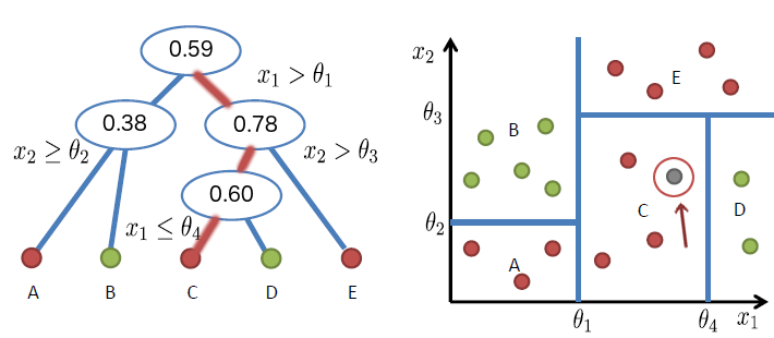
For a decision tree, extracting features contributions means check the path in the tree to reach a given point. In the case of a regression, this path would lead to the value associated with the example that is being scored, while in the binary classification case this path would lead to one of the classes (0 or 1).
Here is an example on binary classification where the grey dot is being classified by the Decision Tree:
Each split on the path moves the prediction up or down, and at each split a single feature is involved. So computing the output difference at each split will indicate the feature influence for that split. For a given feature, we can sum up the contributions for all the splits this is feature is involved. Thus, the output predictions can be written:
P(y = red | x1, x2) = Global_Bias + ∑ contribution_f(x)
On the tree example above, we would have:
- contribution from x1: 0.59
- contribution from x2: -0.18
- global bias: 0.59 which means that x1 has a bigger importance in the classification decision of the grey dot into the red class.
For ensemble methods such as Random Forests and Gradient Boosted Trees, each feature contribution is simply the average of each decision tree's feature contribution.
You can find an implementation of this method here and it has been tested on a house pricing dataset on this notebook.
Yet, even if this method is interesting to identify the important features involved in the prediction, it lacks a sign: it's not possible to know whether x1 should be increased or decreased to switch the outcome of the prediction.
The problem that comes with model independant explanations is that they often can't be compared between each others. Two different models on the same data would lead to two different kind of explanations that would be difficult to compare. So having an explainer that would work on every kind of model would be very useful.
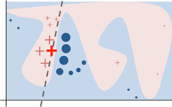
Lime stands for Locally Interpretable Model-agnostic Explanations. It's a local approximation of a complicated model by a interpretable one, namely a linear model.
It is based on this article: "Why Should I Trust You?": Explaining the Predictions of Any Classifier.
Lime starts by sampling many points around the interesting point, then it weights each one of them by a kernel depending of the distance from the original point, and fits a linear model between these samples and their predicted value by the model. So it is a local approximation of the model outcome around the line we want to explain.
The important parameters here are:
kernel_widthwhich controls the width of the weigthing kernel. The smaller, the more local explanations are.num_featuresthat limits the number of displayed features. Note that Lime performs a feature selection before fitting a linear model, so changing this parameter actually changes the output for top features!
An implementation has been released on github by the author. And here is a wrapper that makes the use of Lime a bit easier.
Lime works on various type of data and models. Here you can find several notebooks on text and numerical data:
- On a credit dataset - classification
- On a house prices dataset - regression
- On recipes ingredients dataset - text data
But note that Lime does not work yet on datasets with text and tabular data. In that case you should turn all your data into numbers, including your text, using a count vectorizer or a tfidf for instance.
Another way to locally explain the prediction is to compute the gradient of the model output arount the point. This is quite similar to lime because the derivative is a linear approximation of the model output, but instead of sampling a synthetic dataset, we can recover this model output distribution with a kernel density estimation. Once the desity is recovered using a gaussian kernel for instance, it's then easy to compute the gradient which is then called an explanation vector.
Check this article from the journal of ML research.
In an article from 2009 two researchers described an explanation of individual prediction by making a parallel between coalitions in a game and feature contributions. In Game Theory, it's possible to compute for each play his/her Shapley value, which is an indicator on how much influence in average he would have if he were to engage in a coalition of players. For instance at the Council of the European Union, each state has a number of votes which is proportional to its population, so bigger countries like Germany or France has a greater Shapley value than smaller ones because when they get into a coalition, they increase the coalition's chances to win the vote. And small countries like Luxembourg have a small Shapley value because their small number of votes don't bring much power to the coalition.
So in a group of features, the idea is to determine which feature has the most influence, either alone or combined with other features. Computing the Shapley value for each feature can therefore give a good insight on how much it influences the prediction.
Nonetheless, this methods has a complexity of O(2^n), because it needs to look at each subset of features. This is why the author propose an approximation to the exact Shapley value.


