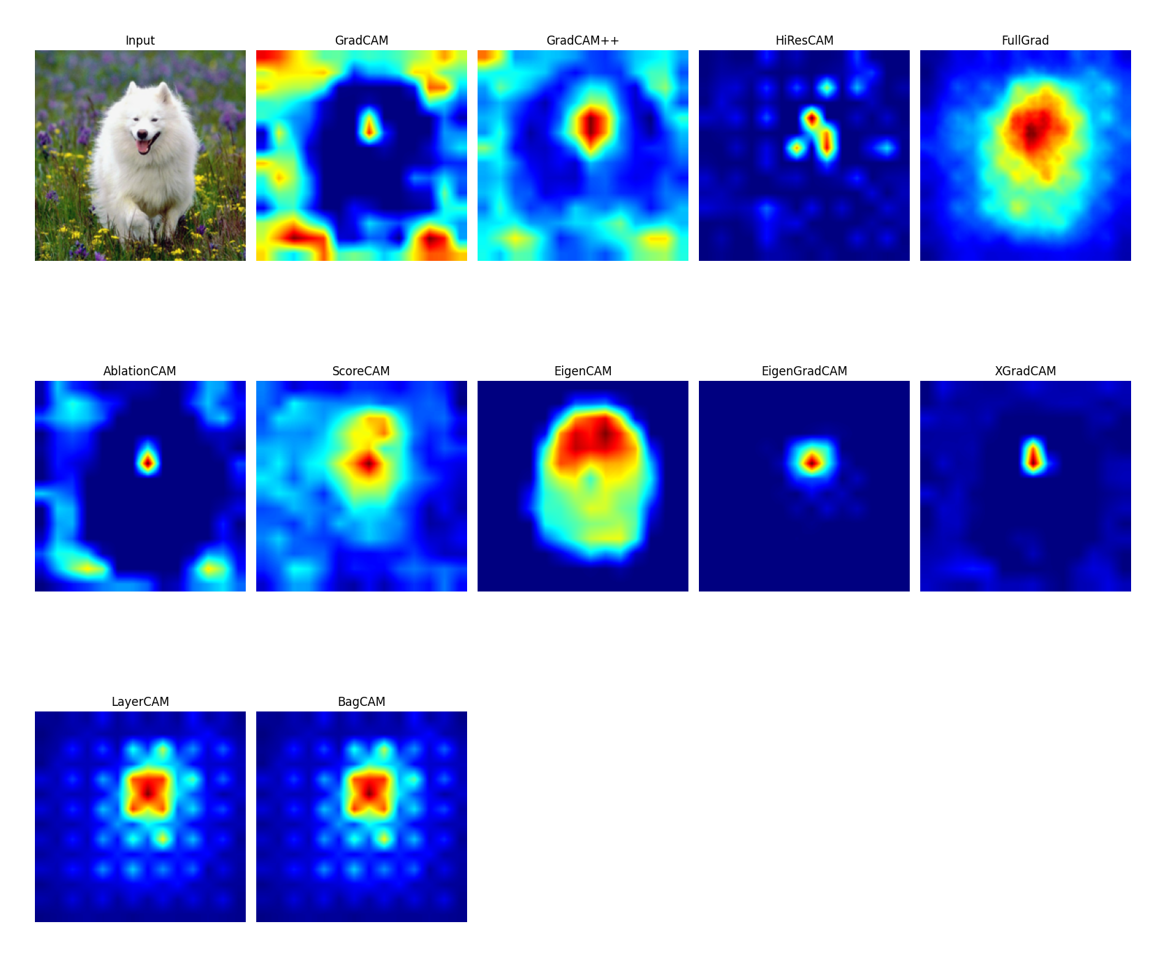
We only consider plug-and-play methods that do not have special requirements on the model architecture and do not need to add modules with learnable parameters or additional training. At the same time, we hope to facilitate weakly-supervised localization and segmentation using attribution results, as well as incorporating them as part of model training (e.g., use the attribution results as additional supervision information). Therefore, all methods use PyTorch tensors for calculations as much as possible, support batch input, and GPU usage.
Since we mainly aim to use attribution results to assist weakly supervised training, localization, segmentation, model distillation and etc., we did not include explainability methods for black-box models like RISE and HISC here.
CNN models: some results of resnet50 from timm, example code at ./gradientss_visualization_examples.py.
Vision/Swin Transformers: gradients visualization methods can be directly used for transformers, the model used here is vit_tiny_patch16_224.augreg_in21k_ft_in1k from timm, example code at ./gradients_visualization_for_transformers_examples.py.
resnet50, the target layer is layer3, example code at ./cam_visualization_examples.py
use attribution.utils.get_reshape_transform when creating the attribution model, example code at ./cam_visualization_for_transformers_examples.py. The target layer used for ViT here is blocks.11.norm1 and that for Swin Transformer is norm.
Currently, some methods are not supported for transformers, such as Ablation-CAM, and the visualization effect is not as good as CNN models since many methods are designed with the concept of feature maps. We will try to add visualization methods that are designed for transformers in the future.
similar to Guided Grad-CAM, any method in the gradient visualization can be combined with CAM visualization, example code at ./combine_cam_and_gradients_visualization_examples.py
example code at ./perturbation_based_attribution_visualization_examples.py
from matplotlib import pyplot as plt
from PIL import Image
import requests
import timm
from timm.data import resolve_model_data_config
from timm.data.transforms_factory import create_transform
import torch

from attribution import BlurIG, GradCAM, CombinedWrapper
from attribution.utils import normalize_saliency, visualize_single_saliency

# Load imagenet labels
IMAGENET_1k_URL = 'https://storage.googleapis.com/bit_models/ilsvrc2012_wordnet_lemmas.txt'
IMAGENET_1k_LABELS = requests.get(IMAGENET_1k_URL).text.strip().split('\n')

# Load model
device = torch.device("cuda" if torch.cuda.is_available() else "cpu")
model = timm.create_model('resnet50', pretrained=True)
model = model.to(device)
model.eval()
config = resolve_model_data_config(model, None)
transform = create_transform(**config)

# Load image
dog = Image.open('examples/dog.png').convert('RGB')
dog_tensor = transform(dog).unsqueeze(0)
H, W = dog_tensor.shape[-2:]
img = transform(dog).unsqueeze(0)

# We support batch input
img = torch.cat([img, img])
img = img.to(device)
output = model(img)
target_index = torch.argmax(output, dim=1).cpu()
print('Predicted:', IMAGENET_1k_LABELS[target_index[0].item()])

# Gradients visualization
blur_ig_kwargs = {'steps': 100,
                  'batch_size': 4,
                  'max_sigma': 50,
                  'grad_step': 0.01,
                  'sqrt': False}
blur_ig_net = BlurIG(model)
blur_ig = normalize_saliency(blur_ig_net.get_mask(img, target_index, **blur_ig_kwargs))

# CAM visualization
gradcam_net = GradCAM(model)
gradcam = normalize_saliency(gradcam_net.get_mask(img, target_index, target_layer='layer3'))

# Combine Gradients and CAM visualization
combined = CombinedWrapper(model, BlurIG, GradCAM)
combined_saliency = normalize_saliency(
    combined.get_mask(img, target_index, target_layer='layer3', **blur_ig_kwargs))

# Visualize
plt.figure(figsize=(16, 5))
plt.subplot(1, 4, 1)
plt.imshow(dog)
plt.title('Input Image')
plt.axis('off')
plt.subplot(1, 4, 2)
visualize_single_saliency(blur_ig[0].unsqueeze(0))
plt.title('Blur IG')
plt.subplot(1, 4, 3)
visualize_single_saliency(gradcam[0].unsqueeze(0))
plt.title('GradCAM')
plt.subplot(1, 4, 4)
visualize_single_saliency(combined_saliency[0].unsqueeze(0))
plt.title('Combined')
plt.tight_layout()
plt.savefig('examples/quick_start.png', bbox_inches='tight', pad_inches=0.5)This is still an ongoing work to implement various attribution methods for image classification models in PyTorch using a unified framework.
- Unify gradient visualization API.
- Implement CAM visualization for CNN models based on known target_layer names.
- Implement CAM for ViT ,Swin Transformer and etc.
- Implement keep positive/negative mask, keep/remove absolute mask metrics. For details, please refer to Fast Axiomatic Attribution for Neural Networks.
- Add LIFT-CAM (ICCV2021), IIA (ICCV2023), Dix (CIKM) and Six (ICDM).
- Unify all APIs.
- Documentation.
This project is inspired by jacobgil/pytorch-grad-cam, PAIR-code/saliency and hummat/saliency. Thanks for their wonderful work.


