Abstract
Insurance is a product sold by insurance companies, which insures the customers stability by transferring loss risk over to the company. The challenge of the insurance companies however is the arbitrary nature of events that cause loss, and many times these losses cost a considerable amount. The fundamental goal of this project is to predict the expected loss of a customer of policy holder based on data we are able to obtain about them. We are asked to produce a pricing model to predict the Pure Premium of policy holders, and we are to be evaluated on the model performance using the Gini coefficient.
Analysis was done using R in this project. Many thanks to my group members Ved Piyush, Zach Gunderson, and Zhuoran Wang for such a pleasurable experience in working together to complete this project, and for the contributions of your hard work and talents to leading our team to win first place in the competition.
Introduction
The scope of this project is to produce predictions for Pure Premium based on auto insurance data. The data was provided to us by folks from Travelers, an Auto Insurance Company. The data comes from one-year insurance policies from 2004 and 2005, with 67856 observations. The relevant response variables in this analysis is clm, numclaims, and claimcst0. For the purpose of this project, the data is split into “T” (training data, consisting of 1/3 of the data), and “V or H” (validation or hold-out data, consisting of 2/3 of the data). The response variables of the “V or H” subset is set to NA, and the goal of this project is to predict the values of claimcst0 for the “V or H” subset. Here is an overview of all the varibles in the data set.
| Variable | Description |
|---|---|
| veh_value | vehicle value, in $10000$s |
| exposure | proportion of year of policy held, ranging from 0 - 1 |
| clm | occurence of claim (0 = No, 1 = Yes) |
| numclaims | number of claims |
| claimcst0 | claim amount (0 if no claim) |
| veh_body | type of vehicle body |
| gender | gender of driver (M, F) |
| area | driver’s area of residence (A, B, C, D, E, F) |
| agecat | driver’s age category, ordinal scale from 1 (young) - 6 (old) |
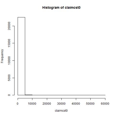
Now let us analyse the distribution of our response variables (Appendix A). The range of claimcst0 (the response varible of interest) is (0,57900) with a mean of 140 and a median of 0. As one can see, the distribution is heavily concentrated at 0, with a relatively small number of observations with a positive value of claimcst0. In fact, 21076 observations had no claim at all, and 1534 had at least one.
Methods
Here we will discuss how we concluded on our regression model, selection of variables and interaction of variables, and the evaluation and validation of the model performance.
Models Considered
The response variable of relevance is claimcst0 or the total cost of claims (loss) in a given exposure period for each policy holder. Let us explore regression models to predict this variable.
Let us first consider the use of the most simplest form of regression: the Ordinary Least Squares. Arguably the most commonly used form of regression, the OLS has several assumptions about the data, one of which is that the distribution of the response variable be of a normal distribution. However, from the figure, we see that the distribution of claimcst0 is heavilty concentrated around 0, followed by several diminishing frequency bars of minimal size.
One solution to resolving the violation of the normality assumption
would be to consider transformations of the response, but to better fit
the nature of the data, it is ideal to consider the use of Generalized
Linear Models, which allows us to select a new distribution that
better fits the response variable.
The folks from Travelers introduced us to the Tweedie Distribution,
which is a family of probability distributions, namely Poisson and Gamma
distributions. The Tweedie distribution allows for the relevant variable
to have a positive mass at zero. while following a continuous
distribution otherwise. So we considered the Tweedie Regression with
a log-link and a variance power of 1.3 (a range of (1,2) corresponds to
the Tweedie distribution, otherwise known as the compound Poisson
model).
However, we were concerned with the idea of using a single model to
predict claimcst0 because this variable is the total cost of claims
summed over multiple claims, and we were unsure whether a single model
would accurately predict this. Instead, after further research, we
decided an alternative approach to modeling claimcst0. We thought of the
cost of claims claimcst0 as a product of the Frequency of claims (in
the given exposure period of the policy) and the Severity of the
claim. So we then considered a Two-Part Model, one that would
predict the Frequency of claims (numclaims), and another that would
predict the average Severity of a claim (claimcst0/numclaims).
We can think of the cost of claims as a prediction of pure premium as
such:
Pure Premium =
Frequency Model
Let us first discuss the first model: the Frequency Model. We want to model the number of claims of policy holders, which takes on discrete values. Therefore the Frequency Model can be modeled using either the Poisson Regression or the Negative Binomial Regression. If the assumptions of the Poisson distribution are held by the data, it is preferred since it is the natural approach to a count data. Let us check some assumptions.
## [1] "Mean of numclaim = 0.072004"
## [1] "Var of numclaim =  0.075403"
For the Poisson distribution, the mean and the variance (
For modeling Frequency, we used log(exposure) as an offset because
log(numclaims/exposure) would theoretically give us the estimated count
in a fixed period of time (in this case one year), but we are only
interested in the numclaims, hence in the model is treated as a response
while offset(log(exposure)) is a predictor. We used exposure as an
offset(log()) instead of as a weight, because when predicting for new
values of x, we would not be able to use exposure as a predictor if it
is treated as a weight in the model.
Let us evaluate the model fit of the full model considering all main
effects and two-way interactions.
## [1] "Deviance = 8165.9794"
## [1] "df = 22403"
We can see that residual deviance is smaller than the degrees of
freedom, which when using the
Severity Model
Now we will move onto the second model: the Severity Model. This model
will take the average claim cost (total claim cost / number of claims)
as the response. From Appendix A, we see that the distribution of the
data has a strong right skewness. Therefore the Severity Model can be
modeled using either the Gamma Regression or the Inverse
Gaussian Regression.
For modeling severity, we only want to consider the data for which there
was a claim, so the appropriate description of the model would be the
mean function of the severity of a claim given that there was a claim.
We considered different distributions for this model, but we found that
the inverse Gaussian model was the best. Our runner-up was the
Gamma regression, but we noticed that the predictions for the Gamma
predictions were too dispersed, and gave us some extreme predictions
(the right-side tail of the prediction distributions were heavy-tailed).
After testing the Inverse Gaussian method (suggested in the book
Generalized Linear Models for Insurance Data, by Heller and Jong), we
saw that the predictions of claimcst0 for the method had more
conservative predictions, so we decided to proceed with Inverse
Gaussian GLM.
Ultimately we used the two-part model, and the prediction of
claimcst0 came from the product of predictions from the Frequency
Model and the predictions from the Severity Model.
Variable Selection
After we decided on the two-part model approach using a Poisson GLM for the Frequency Model and an Inverse Gaussian GLM for the Severity Model, we performed variable selection. We first began with the full main effects and two-way interaction model for the Frequency Model, and the full main effects model for the Severity model (except veh_body). Since we felt this was overparameterizing the models, we used stepwise selection to remove any immediately irrelevant variables and interactions. After, we evaluated the p-values from the model summary and from the results of theAnova function from the car package to consider removal of further variables or the addition of variables previously removed. We evaluated the model performance of adding/deleting one variable at a time by observing the performance of the Gini coefficient from Cross-Validation (more on this later).
The reason we did not consider veh_body as a predictor in either models is because the grouping in veh_body was too sparse. Some categories contained as little as 9 observations, and we decided that model coefficients computed would not be very accurate, perhaps overfitting on those small sample, which would not be appropriate for this analysis.
In addition, we did not consider any interactions in the Severity Model
due to errors in R, either from the model failing to converge or failure
to fit due to overparameterization.
The following models are the final formulas determined through variable
selection (written in R notation):
Frequency .17ex offset(log(exposure)) + factor(agecat) +
area + veh_value + veh_age + veg_value:veh_age + area:veh_value
Severity .17ex gender + veh_age + agecat
Evaluation and Validation
The performance of the Gini coefficient was the ultimate goal of this project, so naturally we used the Gini coefficient to evaluate our model performance. However, simply computing the Gini coefficient on predictions made from the model that used the very same observations (T data) would not be sufficient because if the model were overparameterized or overfitted, we may see an inflated performance of the Gini coefficient on the training data, but the model would perform poorly on a new data (V or H data).
In order to accurately compute a Gini coefficient that would reflect the performance of the true Gini coefficient (or the Gini coefficient we can expect to see for the H data used for the final model performance), we implemented the use of Cross Validation.
Cross Validation
We considered different values of K for the K-fold Cross Validation, but ultimately decided on the 10-fold, as we wanted to keep as much of the data for training for each fold (with 10-fold, we can keep 90% of the data for the model fit). Each run of Cross Validation consisted of 10 iterations, where the data is split into 10 sections, and the model fit on the 90% of the data is tested on the remaining 10%, and obtaining predictions for those 10%. This way, we were able to obtain a full set of predictions from the 10 iterations.
However, we ran into another problem here. After applying a 10-fold Cross Validation the same model several times, we observed a variation in the obtained Gini coefficient for each run of the Cross Validation, as such:
## [1] "Gini coefficients from 10 runs of 10-fold Cross Validation"
##  [1] 0.2088864 0.2121765 0.2048910 0.2138973 0.2110474 0.2100357 0.2135008
##  [8] 0.2135009 0.2117602 0.2108106
## [1] "mean of Gini coefficients"
## [1] 0.2110507
## [1] "sd of Gini coefficients"
## [1] 0.002699676
So to resolve this, we performed the 10-fold Cross Validation 10 times, and obtained the mean of the Gini coefficient from each run, which we then accepted as a sufficient estimate of the true Gini coefficient. We evaluated different varible subsets of the model based on this performance metric.
Bootstrapping
After deciding on the final model and the variable subset, we applied a case-resampling Bootstrapping to recompute model coefficients. The reason for this is to further alleviate the overfitting of the model on the given training data. By allowing bootstrapping to resample the data with replacement and compute coefficients for each iteration, and taking the mean of the coefficients across all iterations, we are able to obtain an unbiased set of coefficients on the same model. For our final predictions, we ran a 500-iteration bootstrap and produced predictions based on the average of the coefficients across the 500 iterations.
This is the comparison of the Frequency Model (first row) vs. the Bootstrapped Frequency Model (second row) with R=20 iterations. We can see the differences in the coefficients.
##      factor(agecat)1 factor(agecat)2 factor(agecat)3 factor(agecat)4
## [1,]       -1.160057       -1.383181       -1.419537       -1.478301
## [2,]       -1.164588       -1.366654       -1.448169       -1.471626
##      factor(agecat)5 factor(agecat)6      areaB      areaC      areaD
## [1,]       -1.727478       -1.625209 -0.2440188 -0.3550608 -0.5632743
## [2,]       -1.744274       -1.594770 -0.2622754 -0.3346268 -0.5316360
##           areaE      areaF  veh_value     veh_age veh_value:veh_age
## [1,] -0.2557080 -0.4185695 -0.2288248 -0.07711640        0.04801158
## [2,] -0.2238647 -0.4737259 -0.2281130 -0.07600485        0.04672113
##      areaB:veh_value areaC:veh_value areaD:veh_value areaE:veh_value
## [1,]       0.1620528       0.1949277       0.2292748      0.10375643
## [2,]       0.1652290       0.1853176       0.2256419      0.08322389
##      areaF:veh_value
## [1,]       0.2099294
## [2,]       0.2236990
Results
Here we would like to discuss the performance of our final mode on the H
data, and interpret the model summaries. First, from our 10 x 10-fold
Cross Validations on the final model, we expected to see a Gini
coefficient of about 0.21. Our result came back as 0.209, off by only
0.001! So we were able to produce a method for accurately predicting the
true Gini coefficient.
Now let us interpret the coefficients from the Frequency Model in
Appendix B. The most informative variables in this model are
factor(agecat), veh_value, the interaction of veh_value
and veh_age, and the interaction of area and veh_value.
From the model output we can say that the youngest age group (agecat
= 1) has the highest rate of claims, and decreases with increasing age,
but then climbs back up slightly for the oldest age group (agecat =
6), which follows our intuition that with age accident rates decrease,
but older folks may have increased rates due to their old age. It is
also interesting to note that the increase of the value of the vehicle
is negatively related with the rate of claim, and that it differs by
area. Another interesting finding is that gender is not a significant
variable here. Males tend to have claim rates just as high as females
do. This is however not the case for the Severity model.
In the Severity Model (Appendix B), we do indeed see that males tend to have a larger Severity than females, by about 24%. We also observed that the older the vehicle was, the higher Severity of claim we expected to see, but with higher driver age, we expected to see a lower Severity. We can justtify this by saying, older cars tend to have larger malfunction rate leading to claims (as we saw in the Frequency Model) and these malfunctions tend to lead to major accidents. We can also say about driver age that younger driver tend to get themselves into larger accidents or claims than older drivers.
Comparison to Runner-up Model
Since we were the winning team, but only by a couple hundredths place (to group 2), we wanted to compare our model with the runner-up model and the different approahces we took. It turned out that they had also used the two-part model, using a Poisson Frequency Model and a Gamma Severity Model. However in addition, they also considered an OLS model to directly predict claimcst0, which according to them seemed to perform at a similar level. They then obtained a weighted average of the predictions from the two approaches as their final submission. I thought this was a very interesting approach, as they did not have to settle for one approach, but compromised by considering both and taking a weighted average. This way, they were also about to consider the weighting allocation that had the best performance. Perhaps if we had considered an approach like this as well, we could have performed even better.
Suggested Improvements to Model
There are several further improvements we could have considered (or would have, if we had more information). For instance, we were not sure what the 0 values in the predictor veh_value meant. We were not sure whether these 0’s truly meant that the value of a vehicle was 0, or if the 0 meant something else (like NULL or MISSING). We ended up using the 0’s in the model, but if we truly understood what those meant we may have changed how we handled those observations.
There were also possible autocorrelation in the data: two individuals
may have had been in the same accident, in which case those two would be
correlated, but from the information provided we would not know. This
could have improved our model by being able to specify a covariance
matrix of some sort and take into account of some autocorrelation.
We also thought about other variables that could have helped improve our
model had we were given the data. For instance, if we had age as a
numeric value rather than categories might have a better predictive
power (gives us more information). Another variable not included in this
data set that could have a high potential for estimating pure premium is
the driver history or record (driving record or any sort of convictions)
which could help estimate how much of a liability the driver could have.
Conclusion
Through exploring various regression models to predict the total claim
loss claimcst0, we found that the two-part model of Pure Premium =
Frequency*Severity was the best approach. We determined this through
evaluating the model performance using the Gini coefficient as the
performance metric. Variable selection was done initially through
stepwise selection, and countless runs of trial-and-error to determine
the best subset of variables for both the Frequency and the Severity
model. Finally, for our final model coefficients, we applied
bootstrapping, and accepted the mean of the coefficients across 500 runs
of bootstrapping to use to predict the response variable of interest
(claimcst0) for the “H” data.
We are quite satisfied with the results, specifically the fact that we
were able to predict so closely the expected Gini coefficient (we
expected to see 0.21, our result was 0.209). I feel that our approach of
the two-part model using the product of the Frequency and Severity Model
was appropriate, and theoretically sound, especially because many
suggest that Pure Premium be computed this way.\
Appendix
A: Response Variable Summary {#a-response-variable-summary .unnumbered}
No claim At least one claim
21076 1534
: Frequency Table of claim vs. no claim (clm) in the training data
| 0 Claims | 1 Claim | 2 Claims | 3 Claims |
|---|---|---|---|
| 21076 | 1443 | 88 | 3 |
: Frequency table of number of claims (numclaims) in the training data
B: Final Model Summaries
## [1] "Summary Frequency Model"
##
## Call:
## glm(formula = numclaims ~ 0 + offset(log(exposure)) + factor(agecat) +
##     area + veh_value + veh_age + veh_value:veh_age + area:veh_value,
##     family = poisson, data = subset(kangtrain))
##
## Deviance Residuals:
##     Min       1Q   Median       3Q      Max
## -0.8100  -0.4473  -0.3437  -0.2273   4.0577
##
## Coefficients:
##                   Estimate Std. Error z value Pr(>|z|)
## factor(agecat)1   -1.16006    0.17606  -6.589 4.42e-11 ***
## factor(agecat)2   -1.38318    0.16997  -8.138 4.03e-16 ***
## factor(agecat)3   -1.41954    0.16979  -8.361  < 2e-16 ***
## factor(agecat)4   -1.47830    0.16887  -8.754  < 2e-16 ***
## factor(agecat)5   -1.72748    0.17682  -9.770  < 2e-16 ***
## factor(agecat)6   -1.62521    0.18110  -8.974  < 2e-16 ***
## areaB             -0.24402    0.13895  -1.756 0.079069 .
## areaC             -0.35506    0.12390  -2.866 0.004159 **
## areaD             -0.56327    0.17151  -3.284 0.001023 **
## areaE             -0.25571    0.19805  -1.291 0.196669
## areaF             -0.41857    0.24618  -1.700 0.089078 .
## veh_value         -0.22882    0.06844  -3.343 0.000828 ***
## veh_age           -0.07712    0.04362  -1.768 0.077097 .
## veh_value:veh_age  0.04801    0.02107   2.278 0.022715 *
## areaB:veh_value    0.16205    0.06804   2.382 0.017229 *
## areaC:veh_value    0.19493    0.05959   3.271 0.001070 **
## areaD:veh_value    0.22927    0.07512   3.052 0.002272 **
## areaE:veh_value    0.10376    0.08769   1.183 0.236714
## areaF:veh_value    0.20993    0.09052   2.319 0.020386 *
## ---
## Signif. codes:  0 '***' 0.001 '**' 0.01 '*' 0.05 '.' 0.1 ' ' 1
##
## (Dispersion parameter for poisson family taken to be 1)
##
##     Null deviance: 20613.1  on 22610  degrees of freedom
## Residual deviance:  8360.2  on 22591  degrees of freedom
## AIC: 11523
##
## Number of Fisher Scoring iterations: 6
## [1] "Summary Severity Model"
##
## Call:
## glm(formula = (claimcst0/numclaims) ~ 0 + gender + veh_age +
##     agecat, family = inverse.gaussian(link = "log"), data = subset(kangtrain,
##     clm > 0))
##
## Deviance Residuals:
##       Min         1Q     Median         3Q        Max
## -0.065718  -0.042700  -0.023112   0.000102   0.116266
##
## Coefficients:
##         Estimate Std. Error t value Pr(>|t|)
## genderF  7.43716    0.17132  43.412  < 2e-16 ***
## genderM  7.65216    0.18625  41.086  < 2e-16 ***
## veh_age  0.12697    0.04548   2.792  0.00531 **
## agecat  -0.09286    0.03323  -2.795  0.00526 **
## ---
## Signif. codes:  0 '***' 0.001 '**' 0.01 '*' 0.05 '.' 0.1 ' ' 1
##
## (Dispersion parameter for inverse.gaussian family taken to be 0.001850414)
##
##     Null deviance: 3.0189e+06  on 1534  degrees of freedom
## Residual deviance: 2.1019e+00  on 1530  degrees of freedom
## AIC: 25425
##
## Number of Fisher Scoring iterations: 10
C: References
Jong, Piet de and Heller, Gillain Z. Generalized Linear Models for Insurance Data. Cambridge. 2008.
D: R Code for Final Predictions
### set working directory, load data, load functions ###
setwd("C:/Users/Riki/Dropbox/UMN Courses/STAT 8051/Travelers/")
kangaroo <- read.csv("Kangaroo.csv")
kangtrain <- subset(kangaroo, split == "T")

SumModelGini <- function(solution, submission) {
  df = data.frame(solution = solution, submission = submission)
  df <- df[order(df$submission, decreasing = TRUE),]
  df
  df$random = (1:nrow(df))/nrow(df)
  df
  totalPos <- sum(df$solution)
  df$cumPosFound <- cumsum(df$solution) # this will store the cumulative number of positive examples found (used for computing "Model Lorentz")
  df$Lorentz <- df$cumPosFound / totalPos # this will store the cumulative proportion of positive examples found ("Model Lorentz")
  df$Gini <- df$Lorentz - df$random # will store Lorentz minus random
  return(sum(df$Gini))
}

NormalizedGini <- function(solution, submission) {
  SumModelGini(solution, submission) / SumModelGini(solution, solution)
}

#cross validation
#since we are using a two-part mode of frequency and severity, in this cv function we specify both models and
#K-fold data divisions are done on both models
#K = # of folds,
cv <- function(fit, fit2 = NULL, data, data2 = NULL, K){
  cost = function(y, yhat) mean((y - yhat)^2)
  n = nrow(data)
  # data divided into K sections of equal size
  if(K > 1) s = sample(rep(1:K, ceiling(nrow(data)/K)),nrow(data)) else
  if(K == 1) s = rep(1, nrow(data))
  glm.y <- fit$y
  cost.0 <- cost(glm.y, fitted(fit))
  ms <- max(s)
  #save model calls
  call <- Call <- fit$call
  if(!is.null(fit2)) call2 <- Call2 <- fit2$call
  #initialize output
  CV <- CV.coef <- NULL
  #progress bar
  pb <- winProgressBar(title = "progress bar", min = 0, max = K, width = 300)
  Sys.time() -> start

  #loop over number of divisions
  for (i in seq_len(ms)) {
    #testing data index
    j.out <- seq_len(n)[(s == i)]
    #training data index
    if(K > 1) j.in <- seq_len(n)[(s != i)] else if (K==1) j.in = j.out
    #fit first model based on training data
    Call$data <- data[j.in, , drop = FALSE];
    d.glm <- eval.parent(Call)
    #prediction on testing data
    pred.glm <- predict(d.glm, newdata=data[j.out,], type="response")
    if(!is.null(fit2) & !is.null(data2)){
      j2.out.data <- merge(data2, data[j.out,])
        if(K > 1) j2.in.data <- merge(data2, data[j.in,]) else if (K==1) j2.in.data = j2.out.data
          #fit second model based on training data
        Call2$data <- j2.in.data
        d.glm2 <- eval.parent(Call2)
        #make prediction on testing data
          pred.glm2 <- predict(d.glm2, newdata=data[j.out,], type="response")
      }
    #produce prediction of two-part model by taking product of predictions from both models
    if(!is.null(fit2)) CV$Fitted = rbind(CV$Fitted, cbind(j.out, pred.glm*pred.glm2)) else
        CV$Fitted = rbind(CV$Fitted, cbind(j.out, pred.glm))
    CV.coef$coef <- rbind(CV.coef$coef, coef(d.glm))
    CV.coef$se <- rbind(CV.coef$se, coef(summary(d.glm))[,2])
    Sys.sleep(0.1); setWinProgressBar(pb, i, title=paste( round(i/K*100, 0),"% done"))
  }#repeat for all K divisions, producing prediction for each observation in data
  close(pb); Sys.time() -> end
  cat("Cross-Validation Time Elapsed: ", round(difftime(end, start, units="secs"),3) ,"seconds \n")
  #re-order predictions to same order as data
  Fitted <- CV$Fitted[order(CV$Fitted[,1]),2]
  #return prediction
  Fitted
}

# bootstrap
library(boot)
bs <- function(formula, data, family, indices) {
  d <- data[indices,] # allows boot to select sample
  fit <- glm(formula, family, data=d)
  return(coef(fit))
}

### fitting the two part model (Frewuency * Severity) ####
#model 1: frequency (or count), final subset of variables
pm.sub <- glm(numclaims ~ offset(log(exposure))+factor(agecat)+area+veh_value+veh_age+
    veh_value:veh_age+area:veh_value, family = poisson, data=subset(kangtrain))
summary(pm.sub)
Count = predict(pm.sub, newdata = kangaroo, type="response")

#apply bootstrapping (500 iterations)
pm.bs <- boot(data=subset(kangtrain), statistic=bs, R=500, formula=formula(pm.sub), family = poisson, parallel="multicore")
#calcualte average of coefficients across 500 iterations
cbind(coef(pm.sub),colMeans(pm.bs$t))

#produce final predictions based on bootstrapped coefficients
pm.sub.bs <- pm.sub
pm.sub.bs$coefficients <- colMeans(pm.bs$t)
Count.bs = predict(pm.sub.bs, newdata = kangaroo, type="response")

#model 2: severity inverse gaussian model, final subset of variables
ivg.sub <- glm((claimcst0/numclaims) ~ gender + veh_age + agecat,
    family=inverse.gaussian(link="log"),data=subset(kangtrain, clm > 0))
Severity = predict(ivg.sub, newdata=kangaroo, type="response")

#apply bootstrapping
ivg.bs <- boot(data=subset(kangtrain, clm > 0 & veh_value>0), statistic=bs, R=500, formula=formula(ivg.sub), family=inverse.gaussian(link="log"), parallel="multicore")
cbind(coef(ivg.sub),colMeans(ivg.bs$t))

#make final predictions based on bootstrapped coefficients
ivg.sub.bs <- ivg.sub
ivg.sub.bs$coefficients <- colMeans(ivg.bs$t)
Severity.bs = predict(ivg.sub.bs, newdata = kangaroo, type="response")

# gini coefficient on the "T" data based on predictions from bootstrapped models
NormalizedGini(kangtrain$claimcst0, predict(pm.sub.bs, newdata=kangtrain, type="response")*predict(ivg.sub.bs, newdata=kangtrain, type="response"))

# gini coefficient on the "T" data based on cross-validation predictions, performed 10 times (10 x 10-fold CV)
cv.ivg <- lapply(1:10, function(x) cv(fit=pm.sub, fit2=gam.sub, data = kangtrain, data2=subset(kangtrain, clm>0), K=10))
#mean of gini coefficients from 10 x 10-fold CV (around .21)
mean(sapply(1:10, function(x) NormalizedGini(kangtrain$claimcst0, cv.ivg[[x]])))
#standard deviation of gini coefficient from 10 X 10-fold CV (around .002)
sd(sapply(1:10, function(x) NormalizedGini(kangtrain$claimcst0, cv.ivg[[x]])))

#write out predictions to .rda file for submission
group1 = as.numeric(subset(Count.bs*Severity.bs, kangaroo$split != "T"))
save(group1, file="group1.rda")