robOcity/song-play-aws-redshift

An ETL pipeline of user song play activity from raw JSON logs file stored S3 buckets to Redshift star schema using SQL and Python.

AWS Redshift Data Warehouse

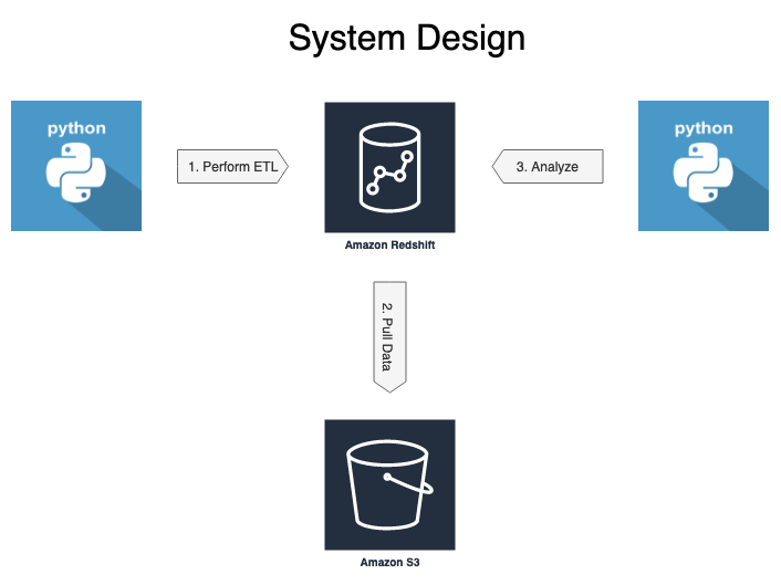
How can you build a simple data pipeline on AWS to support your analytical users? In this repository, I show how using AWS S3 for storage, AWS Redshift to perform ETL and Python to orchestrate it. First, the data are extracted from JSON log files stored on S3 the SQL using Redshift's copy command that creates the staging tables. Next, SQL insert statements transform the data. Finally, I show you how to use the star-schema for analysis.

Files

1. create_tables.py uses sql_queries.py and utils.py to drop (delete) and create all tables. After running this module, the tables have been created and are ready for you to add data.

2. sql_queries.py creates, inserts, and drops all staging and star schema tables. Show how to analyzes the data in the star-schema.

3. utils.py creates connections to a running AWS Redshift instance using data stored in dwh.cfg.

4. events_log_jsonpath.json defines how columns in the events the log file relate to those in the events_staging table — mapping hierarchical JSON data into a flat SQL table. Using columns names from the source file and outputting them in the order specified. See COPY from JSON Format for more information.

5. songplay_log_jsonpath.json selects and orders columns from JSON log files of song play activity into the resulting songplay_staging table. Plays the same role as events_log_jsonpath.json does for the events_staging table.

Table Design

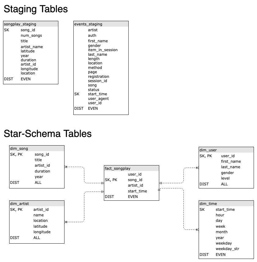
Staging tables support data ingest from online transaction processing systems (OLTP). Here data are extracted from JSON files and inserted into the staging tables using the copy command provided by AWS Redshift. More on that later. Star-schemas are great for supporting analytic workflows utilized by online analytic processing systems (OLAP).

Derived from the code of the open-source PostgreSQL project (see Amazon Redshift and PostgreSQL), Redshift distributes tables allowing for it to operate on the parallel in parallel. Distribution key options include:

• even - spreading data evenly among nodes
• all - an entire copy of the table on every node
• auto - optimized by Redshift
• key - stores data with common key values on a node

The sorting key determines the order of records on each node. Redshift treats primary and foreign keys as suggestions to the query optimizer.

Running

1. Prerequisites:

• You have a S3 bucket with data you want to parse and Redshift cluster up and running.

• You have a security group configured for Redshift allowing for external programmatic access (see Stackoverflow: can't connect to redshift database and Amazon: Troubleshooting Connection Issues in Amazon Redshift). See this Quora post for more information Quora: Can I connect to Redshift using Python?.

• Plus, you the host, port, user name and password stored in a configuration file. Here are the fields your configuration file needs to have.

[CLUSTER]
DB_ENDPOINT=an-endpoint-address-available-on-the-cluster-status-page
DB_NAME=your-db-name
DB_USER=your-db-user
DB_PASSWORD=your-db-users-pw
DB_PORT=5439
CLUSTER_TYPE=multi-node
NUM_NODES=4
NODE_TYPE=dc2.large
AWS_REGION=same-region-as-your-s3-data
CLUSTER_ID=your-clusters-name

[IAM_ROLE]
ROLE=an-iam-role-with-redshift-full-access-ands3-read-only-access
DWH_ROLE_ARN=the-arn-of-this-role

[S3]
LOG_DATA=s3://udacity-dend/log-data
LOG_JSONPATH=s3://udacity-dend/log_json_path.json
SONG_DATA=s3://udacity-dend/song-data

• ** Avoid checking your login credentials into GitHub by having Git ignore your configuration file. To do that you will need to create a .gitignore file at the top-level of you repository. Assuming your configuration file is named dwh.cfg, you need to .cfg, on a line by itself, to your .gitignore file. Or, create a .env folder, add a .env line to .gitignore, and put your configuration file into it. I do both. To easily create a .gitignore file checkout gitignore.io, see examples at github/gitignore, or create your own by referring to gitignore docs.**

Okay, this step was a heavy lift, especially the first time!

1. Run python create_tables.py dropping (deleting) all your exiting tables and re-creating them. These commands run quickly.

2. Run python etl.py1 and type L to extract the data from the log files and insert them into the staging tables. This command took me more than 1 hour to run with four dc2.large nodes in my cluster. The bulk of that time is spent copying the song play data logs.

3. Run python etl.py and type I to transform and load the data from the staging tables into the star-schema tables. This command only took only a few minutes to run on my cluster.

4. Run analytics queries using the Redshift console or other means.

Loading JSON data with COPY

Load data from S3 using Redshift's copy command of JSON data. Let me point out a couple of arguments that I found particularly important.

• truncatecolumns - Shortens long strings to fit into the size of the field in the table. Varchar fields default to 256 bytes -- not characters -- in Redshift.

• epochmillisecs - Parsing time values expressed as UNIX epoch time in milliseconds.

• maxerror - The number of errors allowed before canceling the job. Runtimes for copying the ~400,000 JSON files exceeded an hour with a 4 node cluster.

• compupdate - Turning off compression had little effect upon overall runtimes.

COPY event_staging FROM 's3://udacity-dend/log-data/2018/11/2018-11-11-events.json'
IAM_ROLE 'a-redshift-role-arn'
JSON 's3://dend-util/events_log_jsonpath.json' truncatecolumns
TIMEFORMAT 'epochmillisecs'
REGION 'us-west-2';
COMPUPDATE off
MAXERROR 3;

Providing a JSON paths file allows you to:

• Flatten hierarchical JSON into a flat table

• Select a subset of columns

• Re-order columns

My JSON data was flat, to begin with, so here I am just picking and choosing which columns to take. The names in the jsonpaths file must match the SQL table, and their order must match that of the JSON file. This example uses the event logs of user activity.

{
    "jsonpaths": [
        "$['artist']",
        "$['auth']",
        "$['firstName']",
        "$['gender']",
        "$['itemInSession']",
        "$['lastName']",
        "$['length']",
        "$['level']",
        "$['location']",
        "$['method']",
        "$['page']",
        "$['registration']",
        "$['sessionId']",
        "$['status']",
        "$['ts']",
        "$['userAgent']"
    ]
}

Creating a table

Create the Redshift table using SQL CREATE. I choose to rename columns by using revised column names. JSON data elements inserted into the table based on the order they are defined JSON paths file. The order, number, and types of columns specified in the JSON paths file must match that of the SQL table. For example, itemInSession is inserted into the 5th column of the SQL table and is renamed to item_in_session. This name translation only occurs because I am using a JSON paths file that maps the values between representations.

Redshift runs in parallel and needs to distribute data across the cluster. To do this, Redshift adds:

• A distribution key (DISTKEY) that determines how data partitioned across the cluster's nodes.

• A sorting key (SORTKEY ) that orders the rows on the nodes.

The events_staging table is the largest in this example. I choose a DISTKEY of EVEN to distribution across the cluster. For smaller dimension tables, ALL copies the table to every node and improves performance.

CREATE TABLE IF NOT EXISTS event_staging (
    artist varchar,
    auth varchar,
    first_name varchar,
    gender text,
    item_in_session int,
    last_name text,
    length numeric,
    level text,
    location text,
    method text,
    page text,
    user_id text,
    session_id int,
    status int,
    start_time timestamp,
    user_agent text
)
DISTSTYLE even
SORTKEY (start_time);

Inserting data into fact and dimension tables

Star-schemas are ideal for analytical workflows. Here I show you how to transform data from the staging to dimensional tables.

Initially, I used querys that relied on distinct to assure that the keys to my dimensional tables were unique. Atleast, that is what I had thought. Here is an example of my initial query tranfroming data from a staging to a dimensional table.

INSERT INTO dim_artist (artist_id, name, location, latitude, longitude)
    SELECT DISTINCT sps.artist_id, sps.artist_name, sps.location, sps.longitude, sps.latitude
    FROM songplay_staging AS sps;

It had worked perfectly running on PostgreSQL, but as I discovered, not so much on AWS Redshift. Incredulous? I was too. While PostgreSQL and Redshift share a SQL interface, Redshift stores the column values in consequtive memory locations, whereas Postgres, like most relational databases, store rows. For analytics workflows, where typical queries only use some of the columns, columnar access is much more efficient. Redshift's documentation says that defining primary and foreign keys helps make your queries more efficient but it is up to you to enforce the uniquiness of the keys. So, Redshift assumes your keys are unique once you define a primary or foreign key.

Once I realized that distinct was not working as I expected, I found the following articles that helped my better understand the issue:

• Amazon Redshift – What you need to think before defining primary key

• Redshift PostgreSQL Distinct ON Operator

• DISTINCT ON like functionality for Redshift

First, I tried removing all my primary and foreign keys from my tables but I found the problem continued.

But I was still seeing duplicates in the results to my query.

SELECT artist_id, count(*)
FROM dim_artist
GROUP BY artist_id having count(*) > 1;

Then, I tried using a subquery to order the rows containing duplicates and only take the first one. This worked!_ Here is how I solved the issue for the artist table.

INSERT INTO dim_artist (artist_id, name, location, latitude, longitude)
    (SELECT artist_id, artist_name, location, latitude, longitude
    FROM
        (SELECT artist_id, artist_name, location, latitude, longitude, ROW_NUMBER() OVER (
            PARTITION BY artist_id
            ORDER BY artist_id) AS artist_id_ranked
        FROM songplay_staging
        ORDER BY artist_id)
    WHERE artist_id_ranked = 1)

To analyze the popularity of songs over time, for example, by day of the week, I needed to parse the timestamp and used the extract function to do it. Again, I use the row_number based suquery to remove duplicate values.

INSERT INTO dim_time (start_time, hour, day, week, month, year, weekday, weekday_str)
    SELECT
        start_time,
        extract(hour FROM start_time)      AS hour,
        extract(day FROM start_time)       AS day,
        extract(week FROM start_time)      AS week,
        extract(month FROM start_time)     AS month,
        extract(year FROM start_time)      AS year,
        extract(dayofweek FROM start_time) AS weekday,
        to_char(start_time, 'Dy')          AS weekday_str
    FROM (
    SELECT start_time, user_id, session_id
    FROM (
        SELECT start_time, user_id, session_id, page, ROW_NUMBER() OVER (
            PARTITION BY start_time
            ORDER BY user_id, session_id) AS start_time_ranked
        FROM event_staging
        WHERE page = 'NextSong'
        ORDER BY start_time)
    WHERE start_time_ranked = 1)

Inserting data into the fact table relies on only considering songs that were played and matching them using thier title and duration.

INSERT INTO fact_songplay (user_id, song_id, artist_id, session_id, start_time, level, location, user_agent)
    SELECT es.user_id, saj.song_id, saj.artist_id, es.session_id, es.start_time, es.level, es.location, es.user_agent
    FROM event_staging AS es
    JOIN (
        SELECT ds.song_id, ds.title, ds.duration, da.artist_id, da.name
        FROM dim_song   AS ds
        JOIN dim_artist AS da
    ON ds.artist_id = da.artist_id) AS saj
    ON (es.song = saj.title
    AND es.artist = saj.name
    AND es.length = saj.duration)
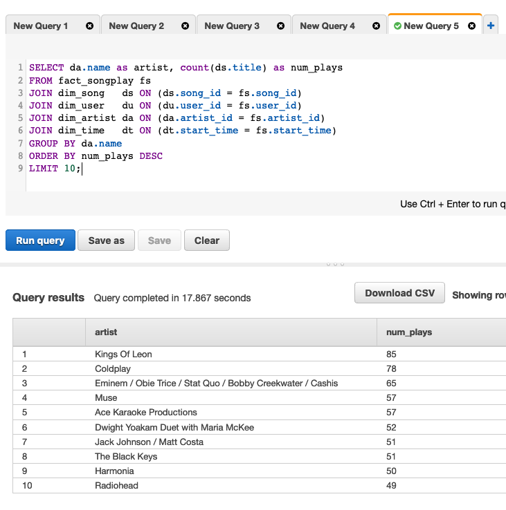
    WHERE es.page = 'NextSong';

Performing analysis

Across the service, who are the top-10 artists?

SELECT da.name as artist, count(ds.title) as num_plays
FROM fact_songplay fs
JOIN dim_song   ds ON (ds.song_id = fs.song_id)
JOIN dim_artist da ON (da.artist_id = fs.artist_id)
GROUP BY da.name
ORDER BY num_plays DESC
LIMIT 10;

Here are the results of this query using the AWS Redshift Query Tool.

Let's find out which songs are most popular by subscriber's gender and whether they have paid or free account.

SELECT du.gender, fs.level, count(distinct(du.user_id))
FROM fact_songplay fs
JOIN dim_user du ON (du.user_id = fs.user_id)
GROUP BY du.gender, fs.level;

How does user activity vary by weekday?

SELECT dt.weekday_str AS Weekday, count(*) AS Count
FROM fact_songplay fs
JOIN dim_time      dt ON (dt.start_time  = fs.start_time)
GROUP BY dt.weekday, dt.weekday_str
ORDER BY dt.weekday;

Useful AWS commands and queries

• Listing the tables in the database using SQL using the Query Tool in Redshift.

SELECT table_schema,table_name
FROM information_schema.tables
WHERE table_schema = 'public'
ORDER BY table_schema,table_name;

• List all files in S3 bucket: aws s3 ls s3://udacity-dend/log-data --recursive

• Display S3 text file: aws s3 cp --quiet s3://udacity-dend/song-data/G/A/W/TRGAWQH128F4222C36.json /dev/stdout

• Debugging copy errors when loading data into staging tables

select * from pg_catalog.stl_load_errors limit 5;

• Debugging redshift errors

from pg_catalog.stl_error
where errcode = '8001';```