👥 Robert Ladwig, Cal Buelo, Ellen Albright, Paul Hanson 📧 contact 💻 more info
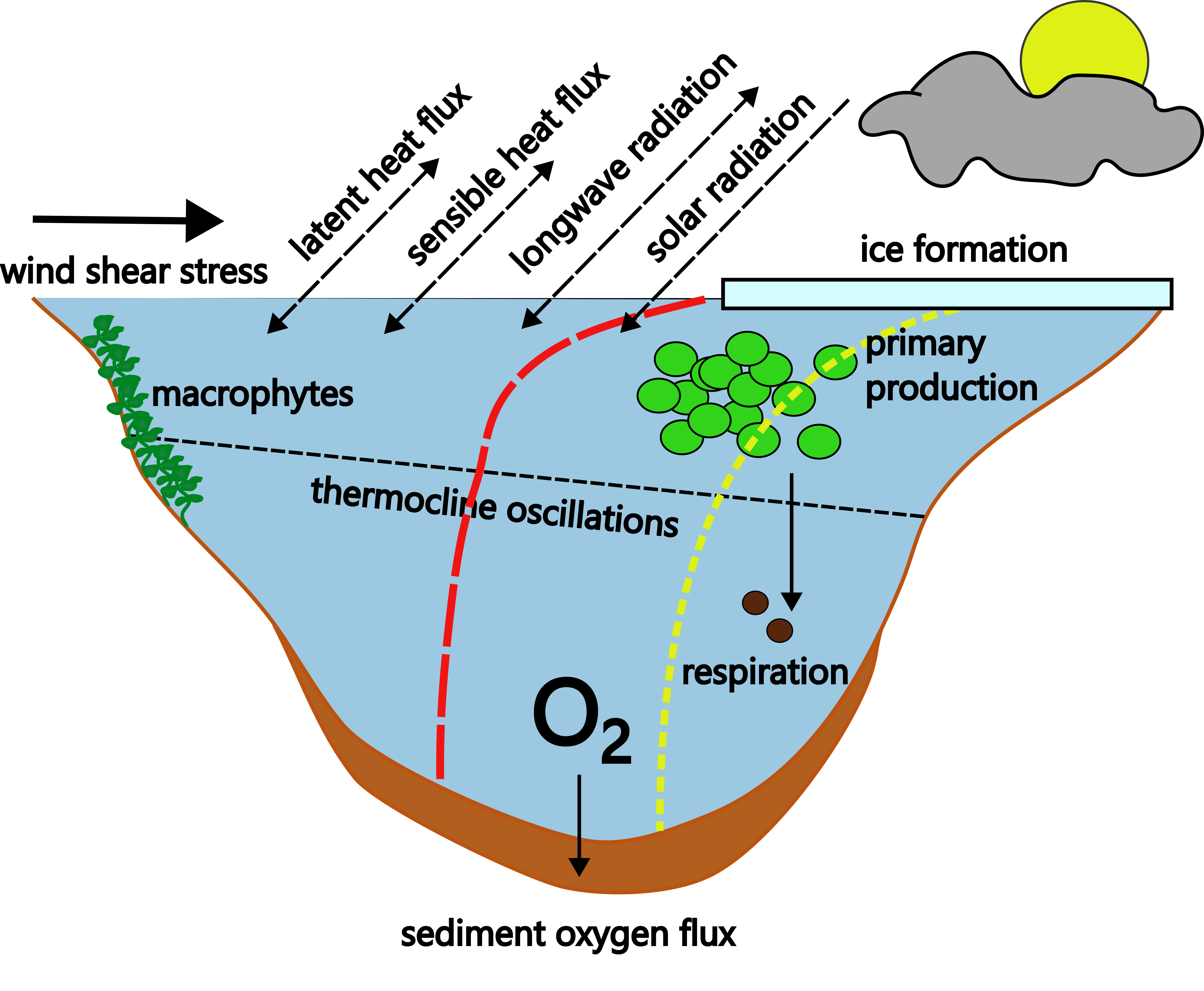
LakeModelR is a R package to run a modularized 1D integral energy model for water temperature dynamics in a lake. The mixing algorithms are based on the MINLAKE (Ford and Stefan 1980, Riley and Stefan 1988, Herb and Stefan 2004) and the MyLake (Saloranta and Andersen 2007) models. Implementations to estimate the incoming and outgoing long-wave heat fluxes were taken from Livingstone and Imboden (1989) and Goudsmit et al. (2002). The latent and sensible heat fluxes were calculated taking into account atmospheric stability using the algorithms by Verburg and Antenucci (2010). The ice algorithms from MyLake (Saloranta and Andersen 2007) were applied to simulate ice formation and melting. Click here for an overview of the model algorithm.
The package can be installed through
#install.packages("remotes")
require(remotes)
remotes::install_github("robertladwig/LakeModelR")
Let us now model a lake's thermal dynamics, potential effects of a macrophyte bed on the attenuation of kinetic energy, and how dissolved oxygen would be created and consumed in an idealized ecosystem.
To test the model code run either example.R or
#' Example workflow to run the 1D integral energy model
#' Long-term Mendota data were obtained from North Temperate Lakes Long Term
#' Ecological Research program (#DEB-1440297)
#' @author: Robert Ladwig
#' @email: ladwigjena@gmail.com

## CLEAN WORKSPACE
rm(list = ls())

## INSTALL PACKAGE
# install.packages("remotes")
# require(remotes)
# remotes::install_github("robertladwig/LakeModelR")

## LOAD PACKAGE(S)
library(LakeModelR)
require(tidyverse)

## GENERAL LAKE CONFIGURATION
zmax = 25 # maximum lake depth
nx = 25 # number of layers we want to have
dt = 3600  # temporal step (here, one hour because it fits boundary data)
dx = zmax/nx # spatial step

## HYPSOGRAPHY OF THE LAKE
hyps_all <- get_hypsography(hypsofile = system.file('extdata', 'bathymetry.csv',
                            package = 'LakeModelR'),
                            dx = dx, nx = nx)

## ATMOSPHERIC BOUNDARY CONDITIONS
meteo_all <- provide_meteorology(meteofile = system.file('extdata', 'meteorology.csv',
                            package = 'LakeModelR'),
                            secchifile = NULL)

### TIME INFORMATION
startingDate <- meteo_all[[1]]$datetime[1]
startTime = 1
endTime = 365 *24 * 3600 # seconds
total_runtime = endTime / 24 / 3600 # days

# INTERPOLATE ATMOSPHERIC BOUNDARY CONDITIONS
meteo = get_interp_drivers(meteo_all = meteo_all,
                           total_runtime = total_runtime,
                           dt = dt,
                           method = "integrate",
                           secchi = F)

## DEFINE INITIAL WATER TEMPERATURE FROM OBSERVED DATA
u_ini <- initial_profile(initfile = system.file('extdata', 'observedTemp.txt',
                            package = 'LakeModelR'),
                            nx = nx, dx = dx,
                            depth = hyps_all[[2]],
                            processed_meteo = meteo_all[[1]])

## RUN THE LAKE MODEL
res <-  run_thermalmodel(u = u_ini,
                          startTime = startTime,
                          endTime =  endTime,
                          ice = FALSE,
                          Hi = 0,
                          iceT = 6,
                          supercooled = 0,
                          kd_light = 0.5,
                          sw_factor = 1.0,
                          zmax = zmax,
                          nx = nx,
                          dt = dt,
                          dx = dx,
                          area = hyps_all[[1]], # area
                          depth = hyps_all[[2]], # depth
                          volume = hyps_all[[3]], # volume
                          daily_meteo = meteo,
                          Cd = 0.0013,
                          scheme = 'implicit')

## SAVE THE RESULTS
temp = res$temp
mixing = res$mixing
ice = res$icethickness
avgtemp = res$average

## POST-PROCESSING OF THE RESULTS
time =  startingDate + seq(1, ncol(temp), 1) * dt
avgtemp = as.data.frame(avgtemp)
colnames(avgtemp) = c('time', 'epi', 'hyp', 'tot', 'stratFlag', 'thermoclineDep')
avgtemp$time = time

## AVERAGE TEMPERATURES IN EPILIMNION AND HYPOLIMNION
ggplot(avgtemp) +
  geom_line(aes(time, epi, col = 'epilimnion')) +
  geom_line(aes(time, hyp, col = 'hypolimnion')) +
  geom_line(aes(time, tot, col = 'total')) +
  theme_minimal()

## CREATE DATAFRAME FOR FULL TEMPERATURE PROFILES
df <- data.frame(cbind(time, t(temp)) )
colnames(df) <- c("time", as.character(paste0(seq(1,nrow(temp)))))
m.df <- reshape2::melt(df, "time")
m.df$time <- time

## CREATE DATAFRAME FOR ICE
df.ice = data.frame('time' = time,
                    'ice_h' = ice)

## HEATMAP OF WATER TEMPERATURE WITH THERMOCLINE DEPTH AND ICE THICKNESS
ggplot(m.df, aes((time), dx*as.numeric(as.character(variable)))) +
  geom_raster(aes(fill = as.numeric(value)), interpolate = TRUE) +
  scale_fill_gradientn(limits = c(-1,30),
                       colours = rev(RColorBrewer::brewer.pal(11, 'Spectral')))+
  theme_minimal()  +xlab('Time') +
  ylab('Depth [m]') +
  labs(fill = 'Temp [degC]')+
  geom_line(data = avgtemp, aes(time, thermoclineDep, col = 'thermocline depth'), linetype = 'dashed', col = 'brown') +
  geom_line(data = df.ice, aes(time, ice_h * (-1), col = 'ice thickness'), linetype = 'solid', col = 'darkblue') +
  scale_y_reverse()

## RUN CUSTOM WATER QUALITY CODE EXAMPLE
require(LakeMetabolizer)

## PROVIDE A FUNCTION FOR YOUR WATER QUALITY BOUNDARY CONDITIONS, HERE FOR OXYGEN
water_quality_boundary_conditions <- function(WQ, TEMP, WIND, AREA, VOLUME, ICE, dt, dx, nx,
                                              EFF_AREA = 0.05,
                                              FVOL = 1.5,
                                              DO2 = NA,
                                              FRED = 1.0,
                                              DELTA_DBL = 1/1000){
  VAR = WQ

  ## SURFACE OXYGEN DEPENDS ON EXCHANGE WITH ATMOPSHERE, HERE WITH PISTON VELOCITY
  k600 =  k600.2.kGAS.base(k.vachon.base(wnd = WIND,
                                         lake.area = max(AREA)),
                                         temperature = TEMP[1], gas = "O2")/86400
  ## DEFINE OXYGEN SATURATION IN ATMOSPHERE
  o2sat = o2.at.sat.base(temp = TEMP[1],
                         altitude = 270)

  ## WE ASSUME LESS EXCHANGE DURING ICE
  if (ICE){
    k600 = 1e-4/86400
  }

  PART_VOLUME <- (VOLUME * 1)/sum(VOLUME)

  ## SURFACE BOUNDARY CONDITION: VOLUME FLUX AND ATMOSPHERIC EXCHANGE
  VAR[1] = VAR[1] +
    ((FVOL/86400) * dt* PART_VOLUME[1] * 1.08^(TEMP[1]-20) +
       (k600 * (o2sat - VAR[1])) * dt/dx * VOLUME[nx])/VOLUME[1]

  ## VOLUME FLUX FOR ALL LAYERS INBETWEEN
  for (i in 2:(nx-1)){
    VAR[i] = VAR[i] +
      (FVOL/86400) * dt * PART_VOLUME[i] * 1.08^(TEMP[i]-20)
  }

  ## BOTTOM BOUNDARY CONDITION: VOLUME FLUX AND SEDIMENT FLUX
  if (is.na(DO2)){
    DO2 = exp((-4.410 + (773.8)/(TEMP[nx] + 273.15) - ((506.4)/(TEMP[nx] + 73.15))^2))/1e4
  }

  BBL_AREA = AREA * EFF_AREA
  VAR[nx] = VAR[nx] +
    ((FVOL/86400) * dt * PART_VOLUME[nx] +
       (- BBL_AREA[nx] * FRED/86400  - BBL_AREA[nx] * (DO2)/DELTA_DBL * VAR[nx]) *
       dt/VOLUME[nx])  * 1.08^(TEMP[nx]-20)

  ## NO CONCENTRATIONS BELOW NULL ARE FEASIBLE
  VAR[which(VAR < 0)] = 0

  return(VAR)
}

## DEFINE INITIAL WATER QUALITY PROFILE
wq_ini <- rep(10, nx)

## RUN THE LAKE MODEL
res <-  run_thermalmodel(u = u_ini,
                         startTime = startTime,
                         endTime =  endTime,
                         ice = FALSE,
                         Hi = 0,
                         iceT = 6,
                         supercooled = 0,
                         kd_light = 0.5,
                         sw_factor = 1.0,
                         zmax = zmax,
                         nx = nx,
                         dt = dt,
                         dx = dx,
                         area = hyps_all[[1]], # area
                         depth = hyps_all[[2]], # depth
                         volume = hyps_all[[3]], # volume
                         daily_meteo = meteo,
                         Cd = 0.0013,
                         scheme = 'implicit',
                         water.quality = TRUE,
                         wq = wq_ini)

## SAVE THE RESULTS
ice = res$icethickness
avgtemp = res$average
dissoxygen = res$water.quality

## POST-PROCESSING OF THE RESULTS
time =  startingDate + seq(1, ncol(temp), 1) * dt
avgtemp = as.data.frame(avgtemp)
colnames(avgtemp) = c('time', 'epi', 'hyp', 'tot', 'stratFlag', 'thermoclineDep')
avgtemp$time = time

df.dissoxygen <- data.frame(cbind(time, t(dissoxygen)) )
colnames(df.dissoxygen) <- c("time", as.character(paste0(seq(1,nrow(dissoxygen)))))
m.df.dissoxygen <- reshape2::melt(df.dissoxygen, "time")
m.df.dissoxygen$time <- time

## CREATE DATAFRAME FOR ICE
df.ice = data.frame('time' = time,
                      'ice_h' = ice)

## HEATMAP OF DISSOLVED OXYGEN WITH THERMOCLINE DEPTH AND ICE THICKNESS
ggplot(m.df.dissoxygen, aes((time), dx*as.numeric(as.character(variable)))) +
    geom_raster(aes(fill = as.numeric(value)), interpolate = TRUE) +
    scale_fill_gradientn(limits = c(0,15),
                         colours = rev(RColorBrewer::brewer.pal(9, 'YlGnBu')))+
    theme_minimal()  +xlab('Time') +
    ylab('Depth [m]') +
    labs(fill = 'Diss. Oxygen [gm-3]')+
    geom_line(data = avgtemp, aes(time, thermoclineDep, col = 'thermocline depth'), linetype = 'dashed', col = 'brown') +
    geom_line(data = df.ice, aes(time, ice_h * (-1), col = 'ice thickness'), linetype = 'solid', col = 'darkblue') +
    scale_y_reverse()
References:
Ford, D.E., and H.G. Stefan. 1980. Thermal predictions using an integral energy model. J. Hydraul. Div. ASCE 106(1). 39-55
Goudsmit, G.H., H. Burchard, F. Peeters, and A. Wüst. 2002. Application of k-e turbulence models to enclosed basins: The role of internal seiches. Journal of Geophysical Research 107. C12. 3230. doi:10.1029/2001JC000954
Herb, W.R., and H.G. Stefan. 2004. Temperature Stratification and Mixing Dynamics in a Shallow Lake With Submersed Macrophytes. Lake and Reservoir Management 20. 4. 296-308. doi:10.1080/07438140409354159
Livingstone, D., and D. Imboden. 1989. Annual heat balance and equilibrium temperature of Lake Aegeri, Switzerland. Aquat. Sci. 51
Riley, M., and H.G. Stefan. 1988. MINLAKE: A dynamic lake water quality simulation model. Ecol. Model. 43. 155-182
Saloranta, T.M., and T. Andersen. 2007. MyLake – A multi-year lake simulation model code suitable for uncertainty and sensitivity analysis simulation. Ecol. Model. 207. 1. 45-60. doi:https://doi.org/10.1016/j.ecolmodel.2007.03.018
Verburg, P., and J.P. Antenucci. 2010. Persistent unstable atmospheric boundary layer enhances sensible and latent heat loss in a tropical great lake: Lake Tanganyika. Journal of Geophysical Research Atmospheres 115. D11. doi:https://doi.org/10.1029/2009JD012839

