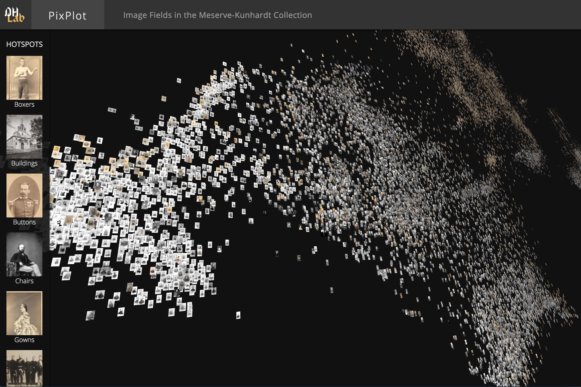
This repository contains code that can be used to visualize tens of thousands of images in a two-dimensional projection within which similar images are clustered together. The image analysis uses Tensorflow's Inception bindings, and the visualization layer uses a custom WebGL viewer.
See the change log for recent updates.
We maintain several platform-specific installation cookbooks online.
Broadly speaking, to install the Python dependencies, we recommend you install Anaconda and then create a conda environment with a Python 3.7 runtime:
conda create --name=3.7 python=3.7
source activate 3.7
Then you can install the dependencies by running:
bash
pip install https://github.com/yaledhlab/pix-plot/archive/master.zip
The website that PixPlot eventually creates requires a WebGL-enabled browser.
If you have a WebGL-enabled browser and a directory full of images to process, you can prepare the data for the viewer by installing the dependencies above then running:
pixplot --images "path/to/images/*.jpg"To see the results of this process, you can start a web server by running:
# for python 3.x
python -m http.server 5000

# for python 2.x
python -m SimpleHTTPServer 5000
The visualization will then be available at http://localhost:5000/output.
To acquire some sample data with which to build a plot, feel free to use some data prepared by Yale's DHLab:
pip install image_datasetsThen in a Python script:
import image_datasets
image_datasets.oslomini.download()
The .download() command will make a directory named datasets in your current working directory. That datasets directory will contain a subdirectory named 'oslomini', which contains a directory of images and another directory with a CSV file of image metadata. Using that data, we can next build a plot:
pixplot --images "datasets/oslomini/images/*" --metadata "datasets/oslomini/metadata/metadata.csv"If you need to plot more than 100,000 images but don't have an expensive graphics card with which to visualize huge WebGL displays, you might want to specify a smaller "cell_size" parameter when building your plot. The "cell_size" argument controls how large each image is in the atlas files; smaller values require fewer textures to be rendered, which decreases the GPU RAM required to view a plot:
pixplot --images "path/to/images/*.jpg" --cell_size 10The UMAP algorithm is particularly sensitive to three hyperparemeters:
--min_dist: determines the minimum distance between points in the embedding
--n_neighbors: determines the tradeoff between local and global clusters
--metric: determines the distance metric to use when positioning points
UMAP's creator, Leland McInnes, has written up a helpful overview of these hyperparameters. To specify the value for one or more of these hyperparameters when building a plot, one may use the flags above, e.g.:
pixplot --images "path/to/images/*.jpg" --n_neighbors 2If installed and available, PixPlot uses Hierarchical density-based spatial clustering of applications with noise, a refinement of the earlier DBSCAN algorithm, to find hotspots in the visualization. You may be interested in consulting this explanation of how HDBSCAN works.
Tip: If you are using HDBSCAN and find that PixPlot creates too few (or only one) 'automatic hotspots', try lowering the --min_cluster_size from its default of 20. This often happens with smaller datasets (less than a few thousand.)
If HDBSCAN is not available, PixPlot will fall back to scikit-learn's implementation of KMeans.
If you have metadata associated with each of your images, you can pass in that metadata when running the data processing script. Doing so will allow the PixPlot viewer to display the metadata associated with an image when a user clicks on that image.
To specify the metadata for your image collection, you can add --metadata=path/to/metadata.csv to the command you use to call the processing script. For example, you might specify:
pixplot --images "path/to/images/*.jpg" --metadata "path/to/metadata.csv"Metadata should be in a comma-separated value file, should contain one row for each input image, and should contain headers specifying the column order. Here is a sample metadata file:
| filename | category | tags | description | permalink | Year |
|---|---|---|---|---|---|
| bees.jpg | yellow | a|b|c | bees' knees | https://... | 1776 |
| cats.jpg | dangerous | b|c|d | cats' pajamas | https://... | 1972 |
The following column labels are accepted:
| Column | Description |
|---|---|
| filename | the filename of the image |
| category | a categorical label for the image |
| tags | a pipe-delimited list of categorical tags for the image |
| description | a plaintext description of the image's contents |
| permalink | a link to the image hosted on another domain |
| year | a year timestamp for the image (should be an integer) |
| label | a categorical label used for supervised UMAP projection |
| lat | the latitudinal position of the image |
| lng | the longitudinal position of the image |
If you would like to process images that are hosted on a IIIF server, you can specify a newline-delimited list of IIIF image manifests as the --images argument. For example, the following could be saved as manifest.txt:
https://manifests.britishart.yale.edu/manifest/40005
https://manifests.britishart.yale.edu/manifest/40006
https://manifests.britishart.yale.edu/manifest/40007
https://manifests.britishart.yale.edu/manifest/40008
https://manifests.britishart.yale.edu/manifest/40009
One could then specify these images as input by running pixplot --images manifest.txt --n_clusters 2
| Link | Image Count | Collection Info | Browse Images | Download for PixPlot |
|---|---|---|---|---|
| NewsPlot: 1910-1912 | 24,026 | George Grantham Bain Collection | News in the 1910s | Images, Metadata |
| Bildefelt i Oslo | 31,097 | oslobilder | Advanced search, 1860-1924 | Images, Metadata |
The DHLab would like to thank Cyril Diagne and Nicolas Barradeau, lead developers of the spectacular Google Arts Experiments TSNE viewer, for generously sharing ideas on optimization techniques used in this viewer, and Lillianna Marie for naming this viewer PixPlot.
