- INDEX
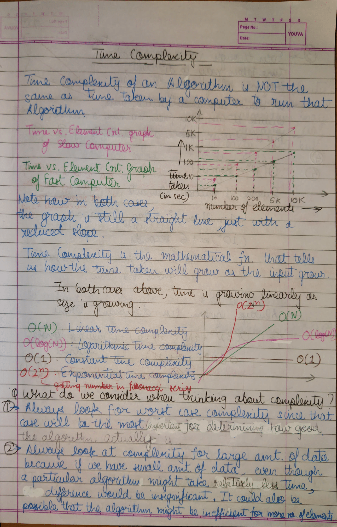
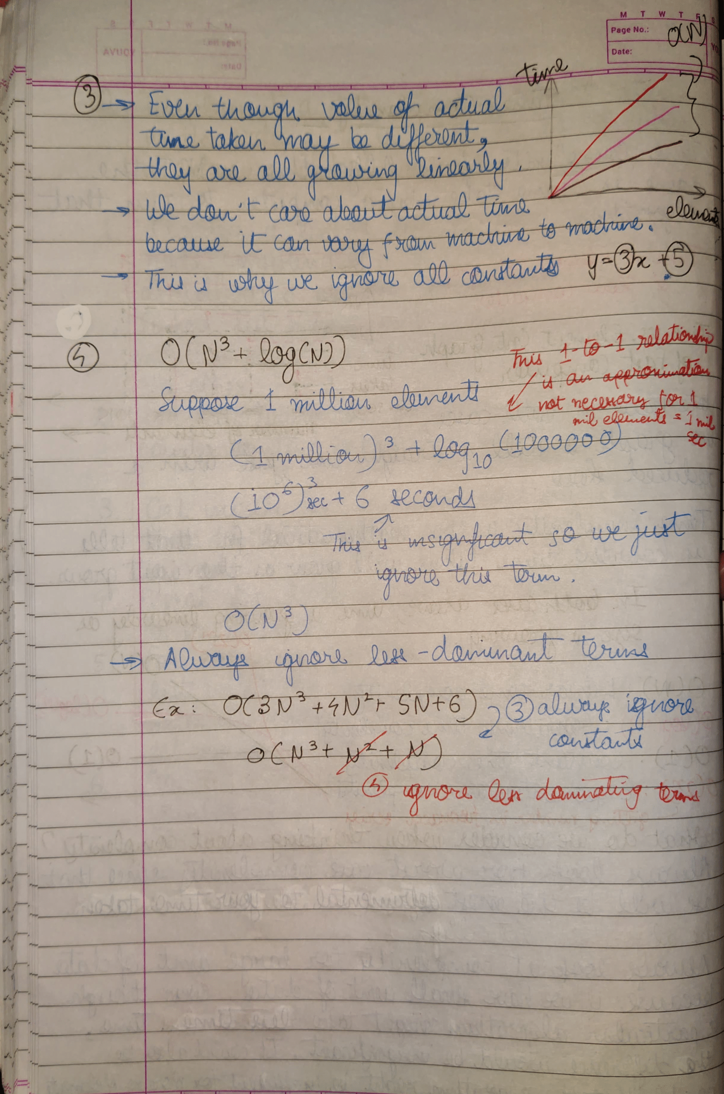
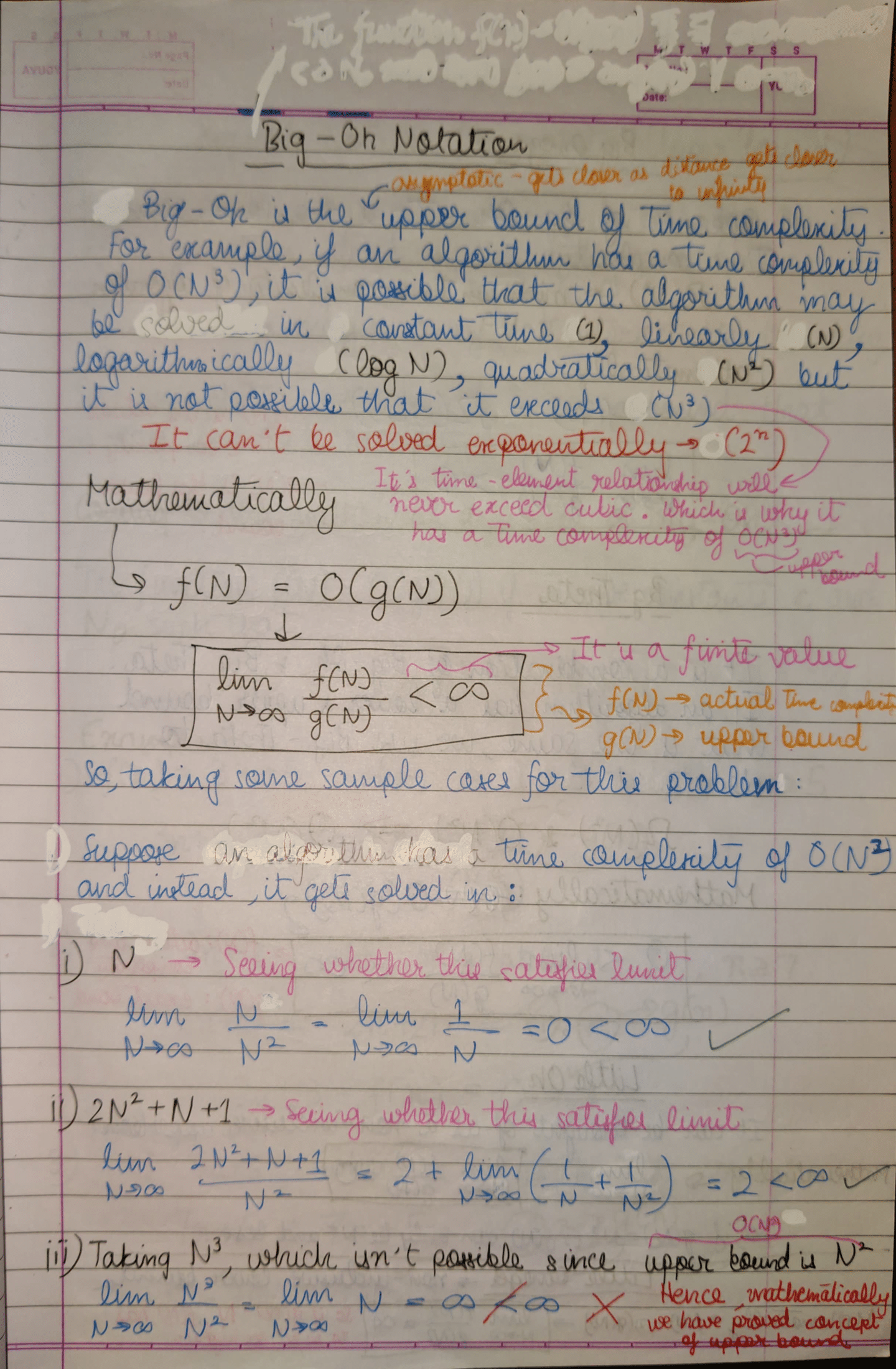
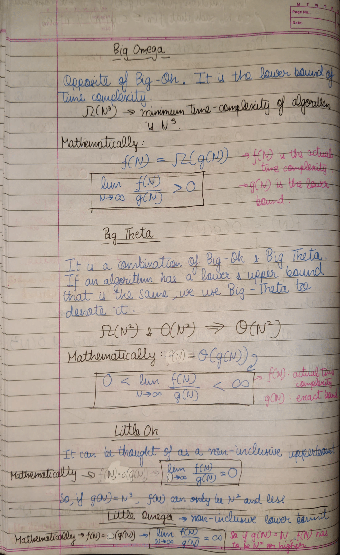
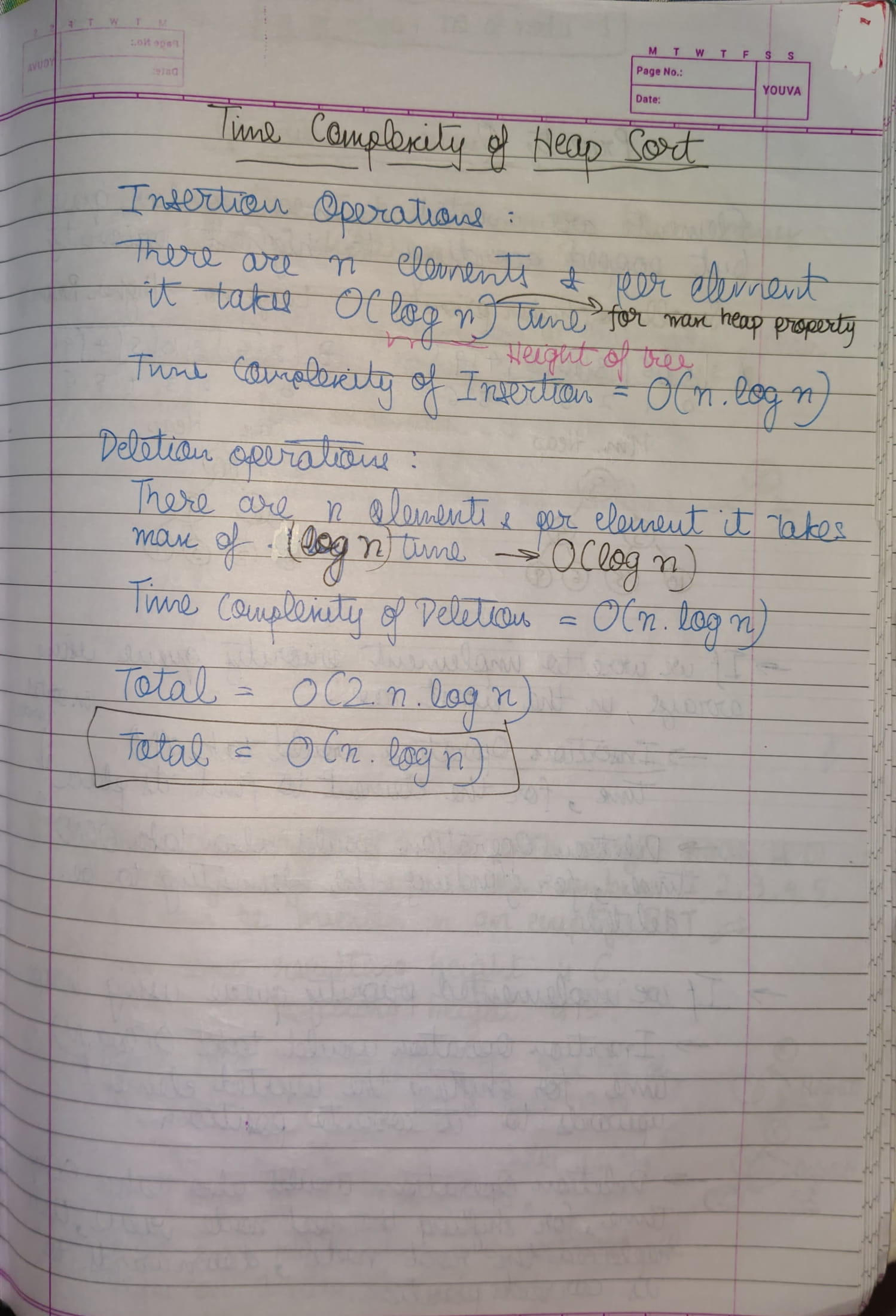
- Time Complexity
- Space Complexity
- Recursion
- Dynamic Programming
- Arrays
- Abstract Data Types
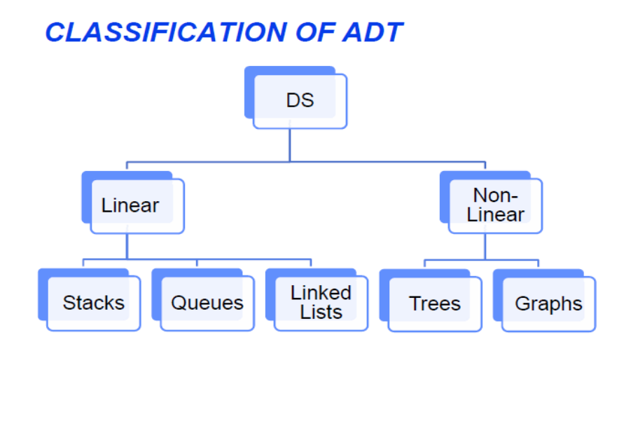
- Linear Abstract Datatypes
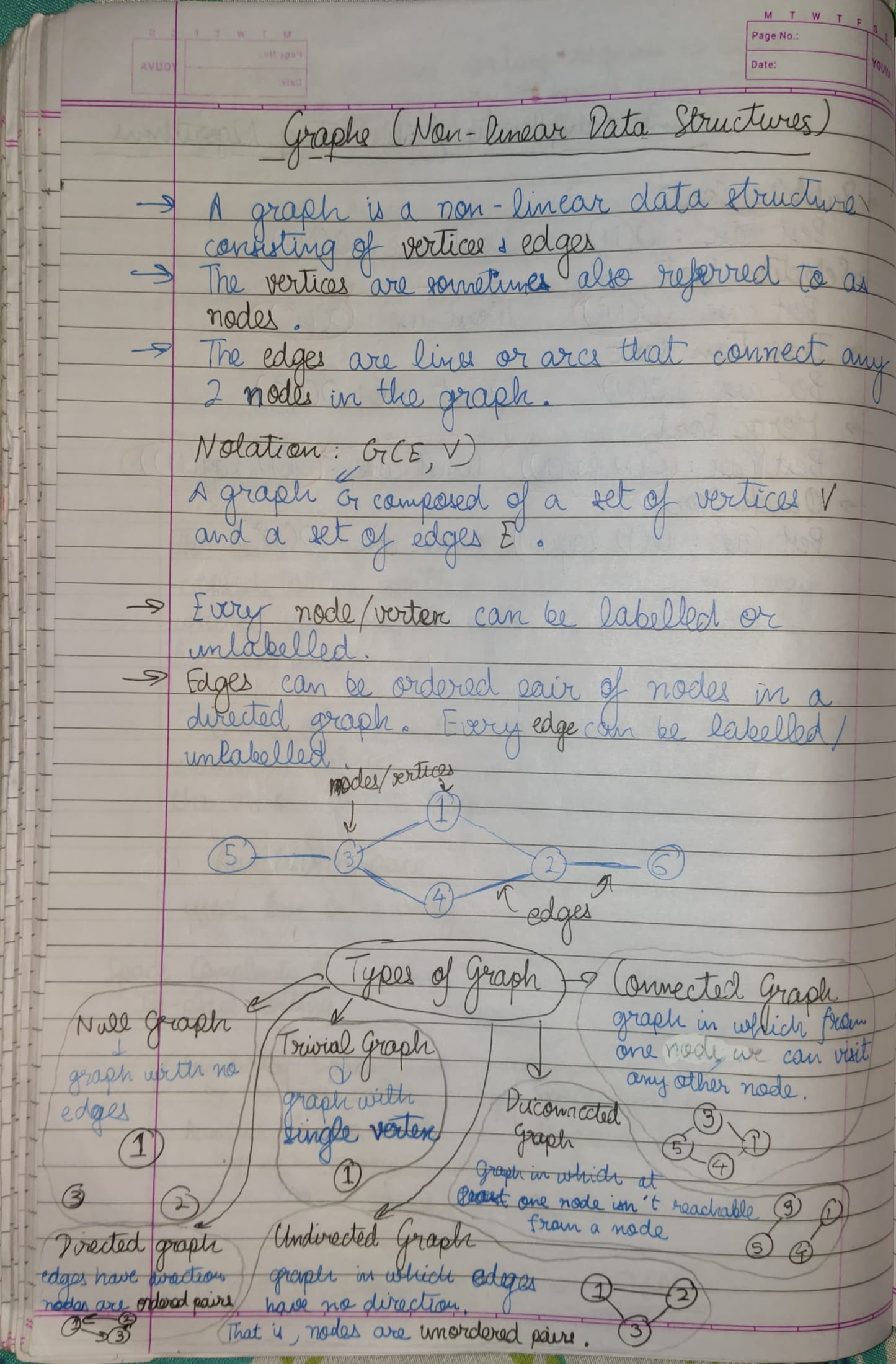
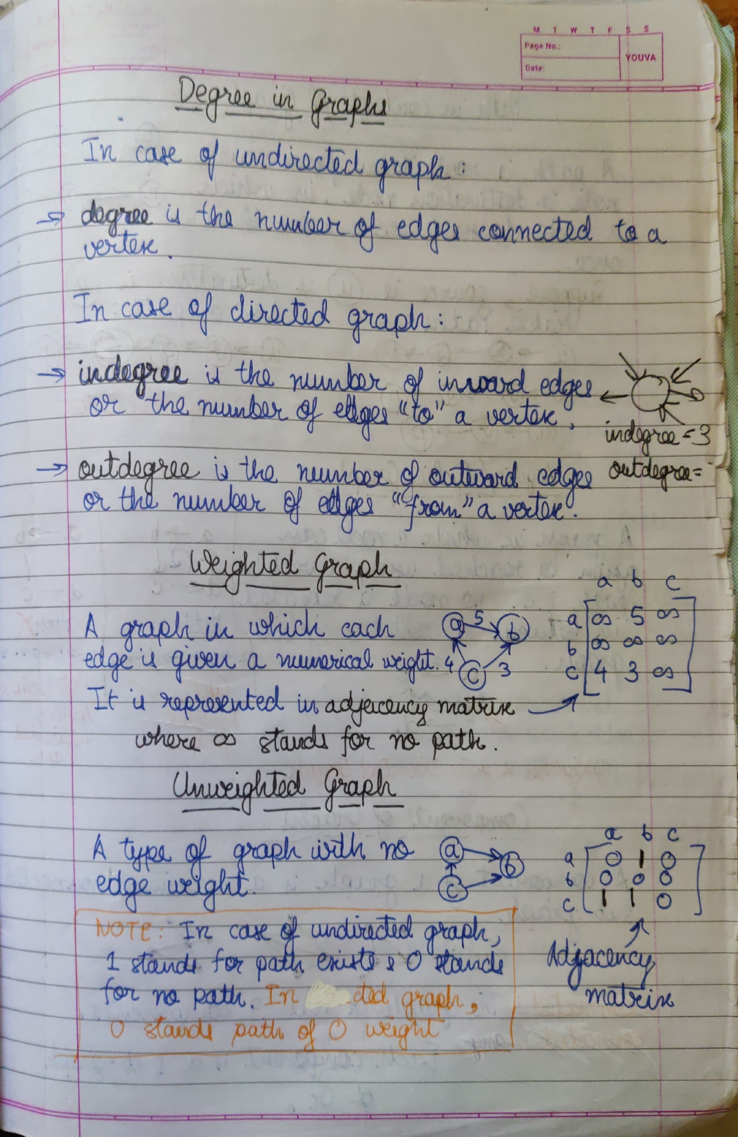
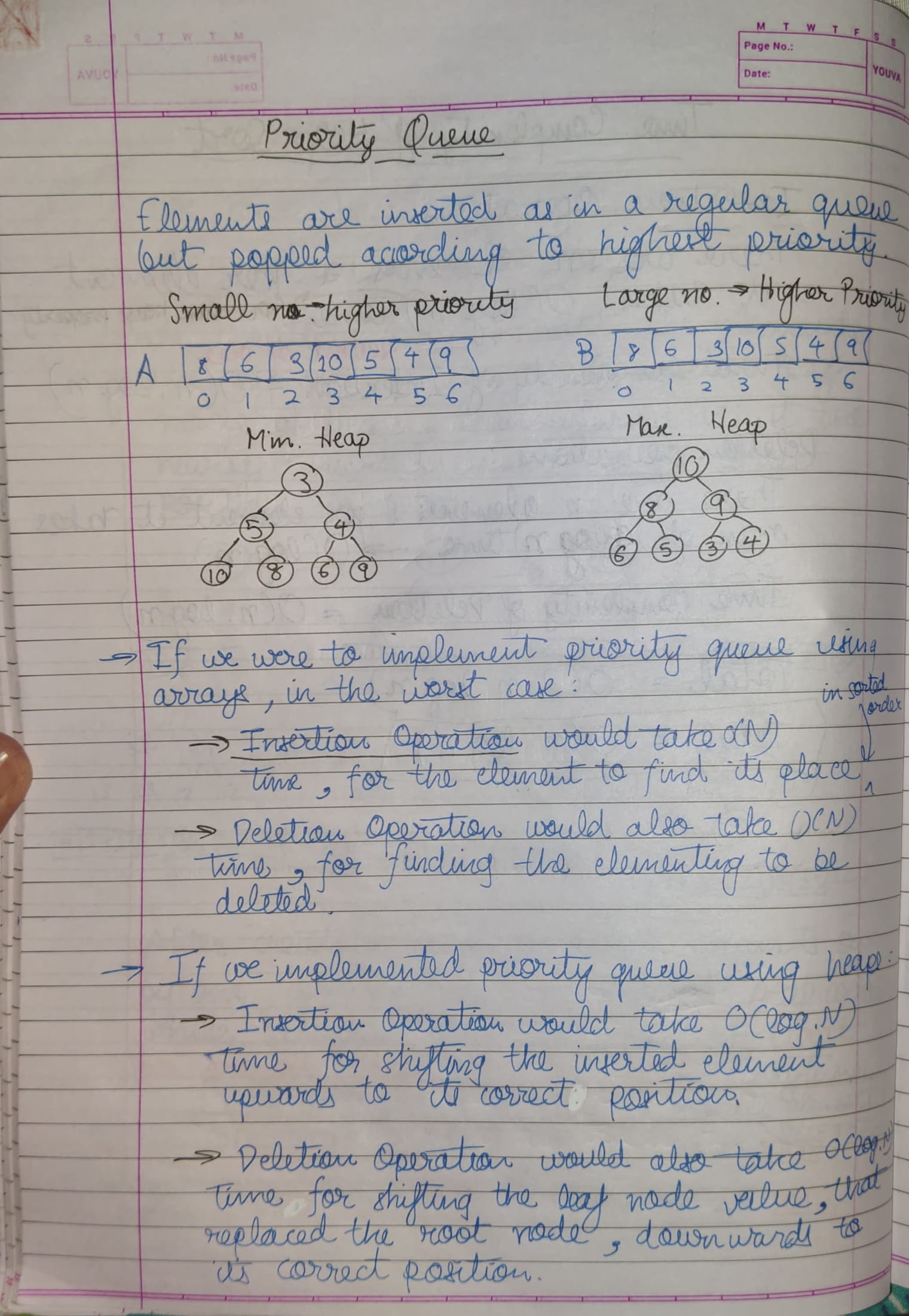
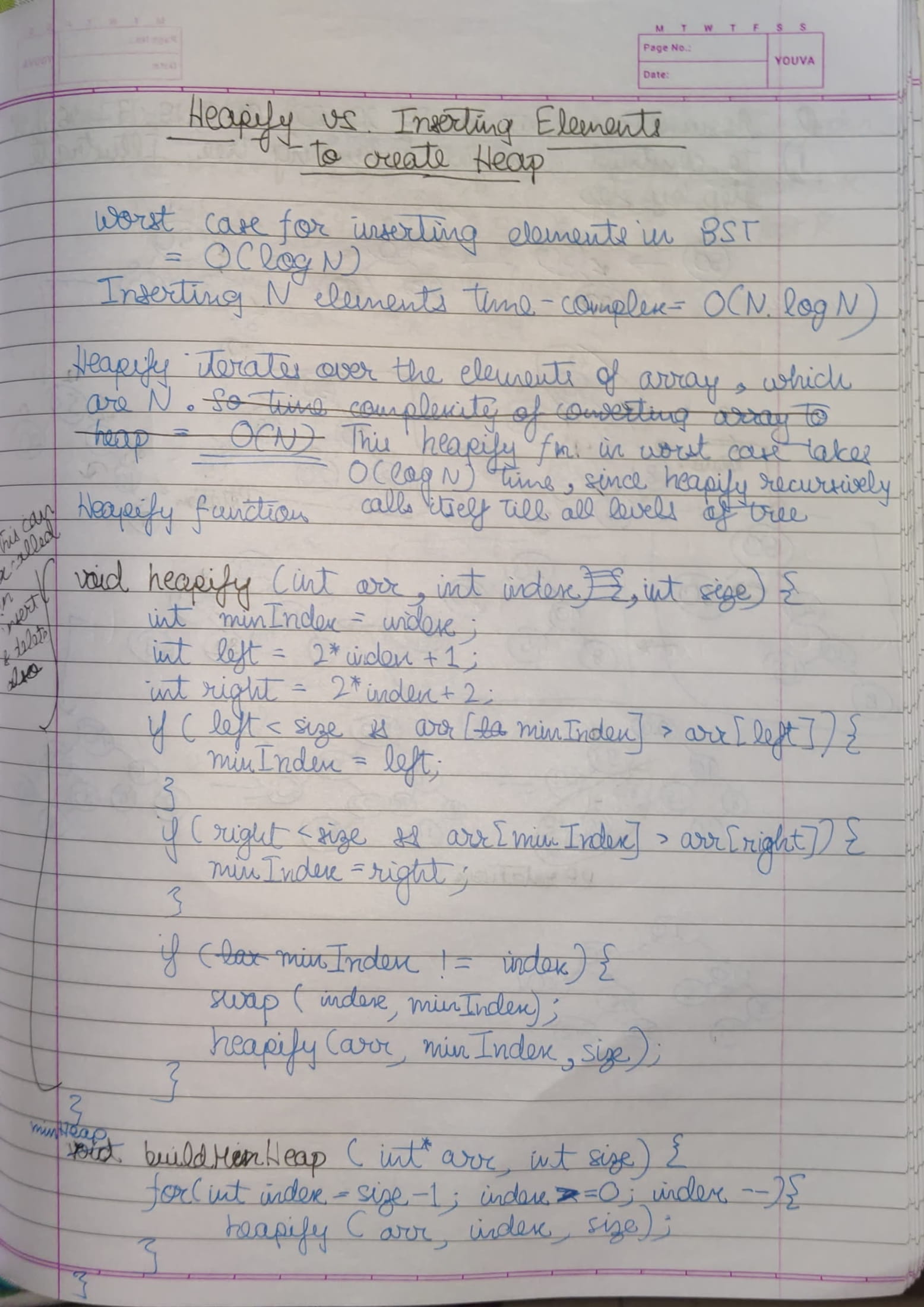
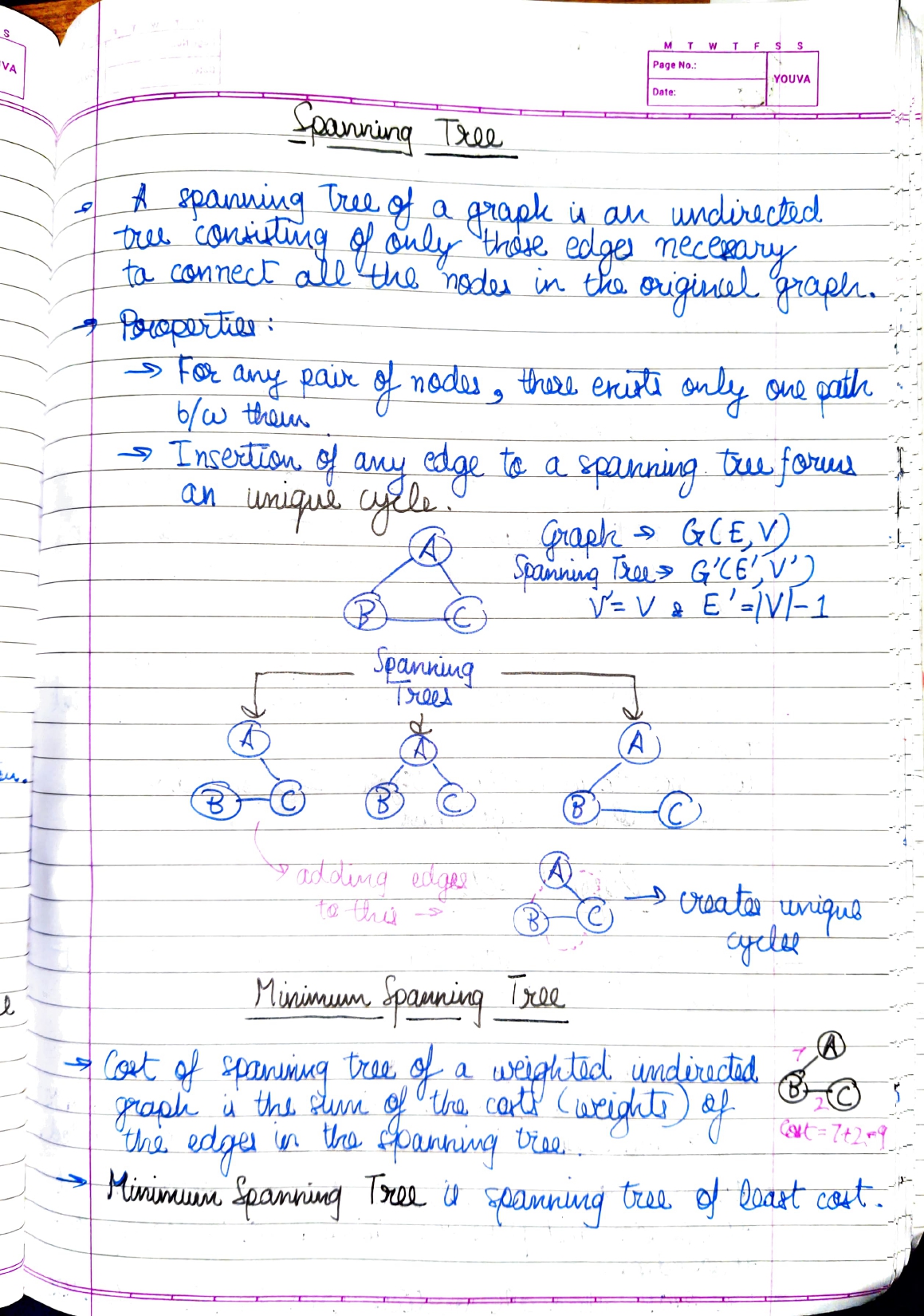
- Non-Linear Abstract Data Types
- Sorting Algorithms
- Searching Algorithms
- Binary Search
- Rotated Binary Search
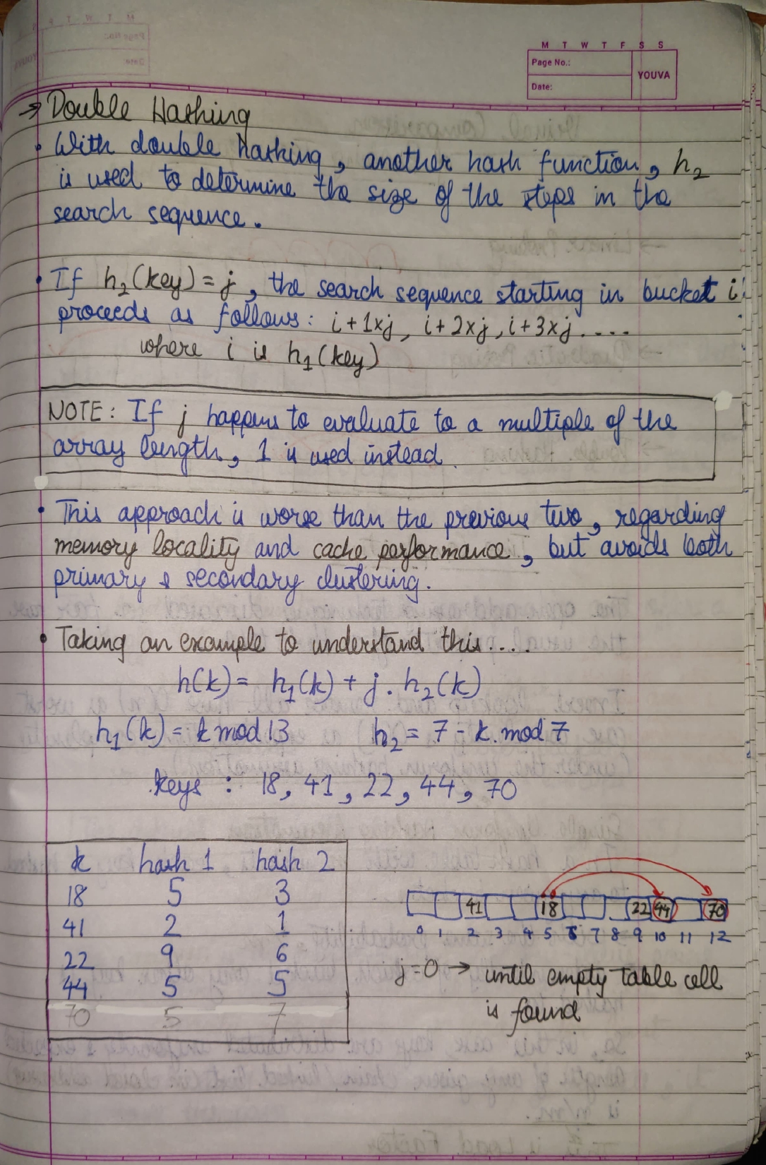
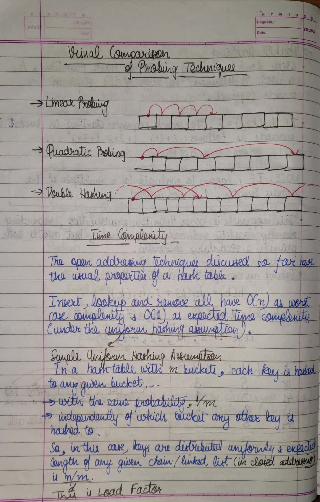
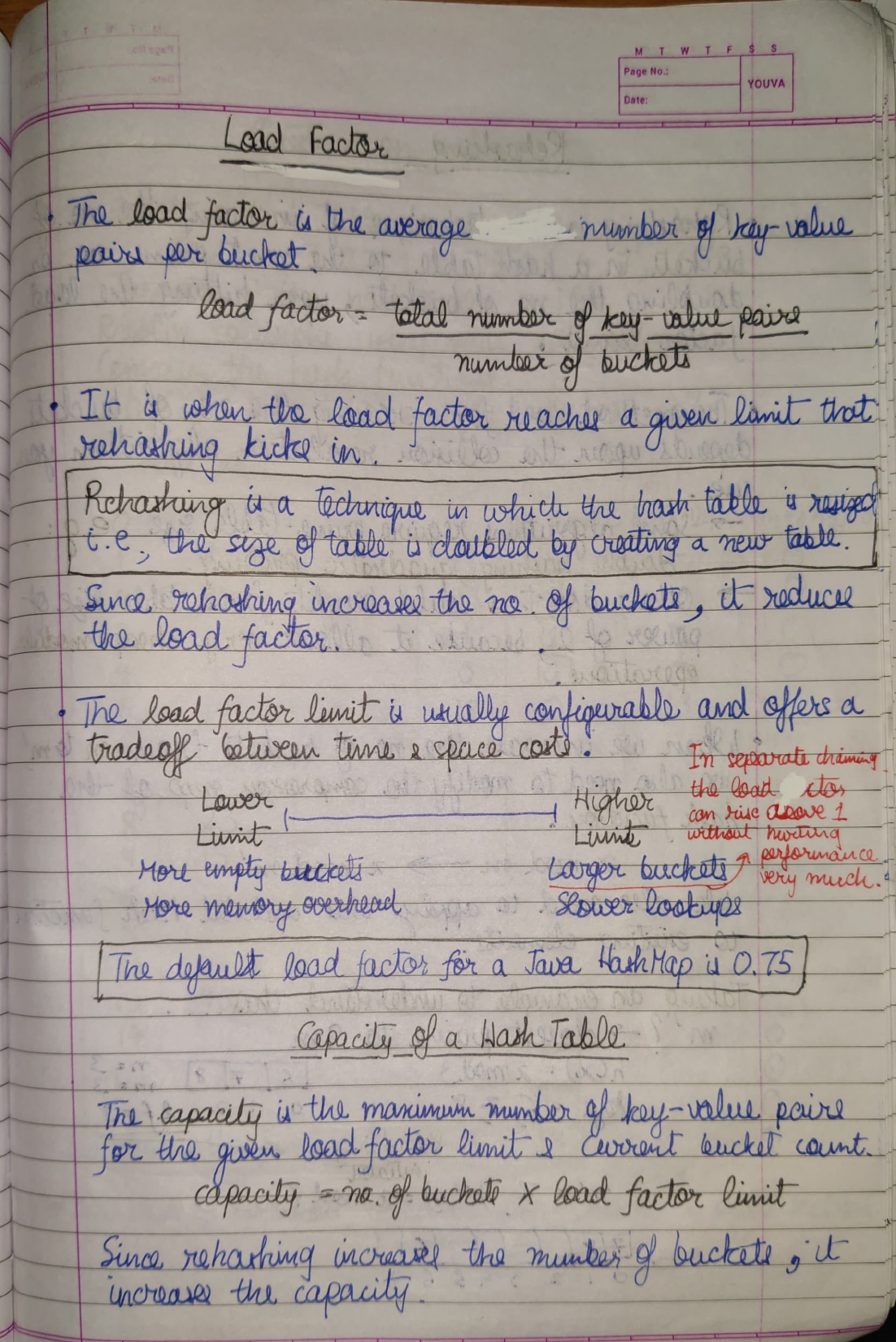
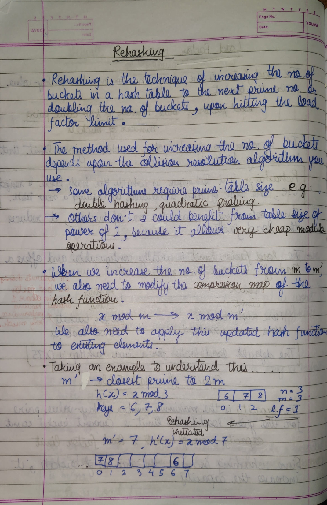
- Hashing (using Hash Functions :P)
- Tips & Tricks for DSA
- Method for Artifically Changing Base Fast (to a base below 10)
- TODO
Access it here.
Space Complexity of an algorithm is the total space taken by an algorithm withm respect to the input size. Space complexity includes both Auxiliary space and space used by input.
Auxiliary space is the extra space or the temporary space used by an algorithm.
We can't really do anything about the input we are taking, but we can choose what algorithm to use, depending on which takes up the least amount of memory.
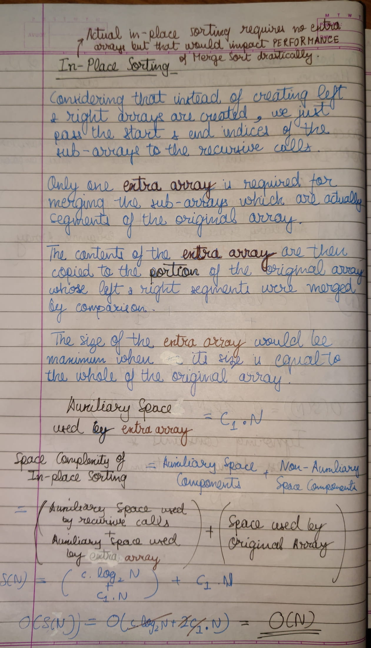
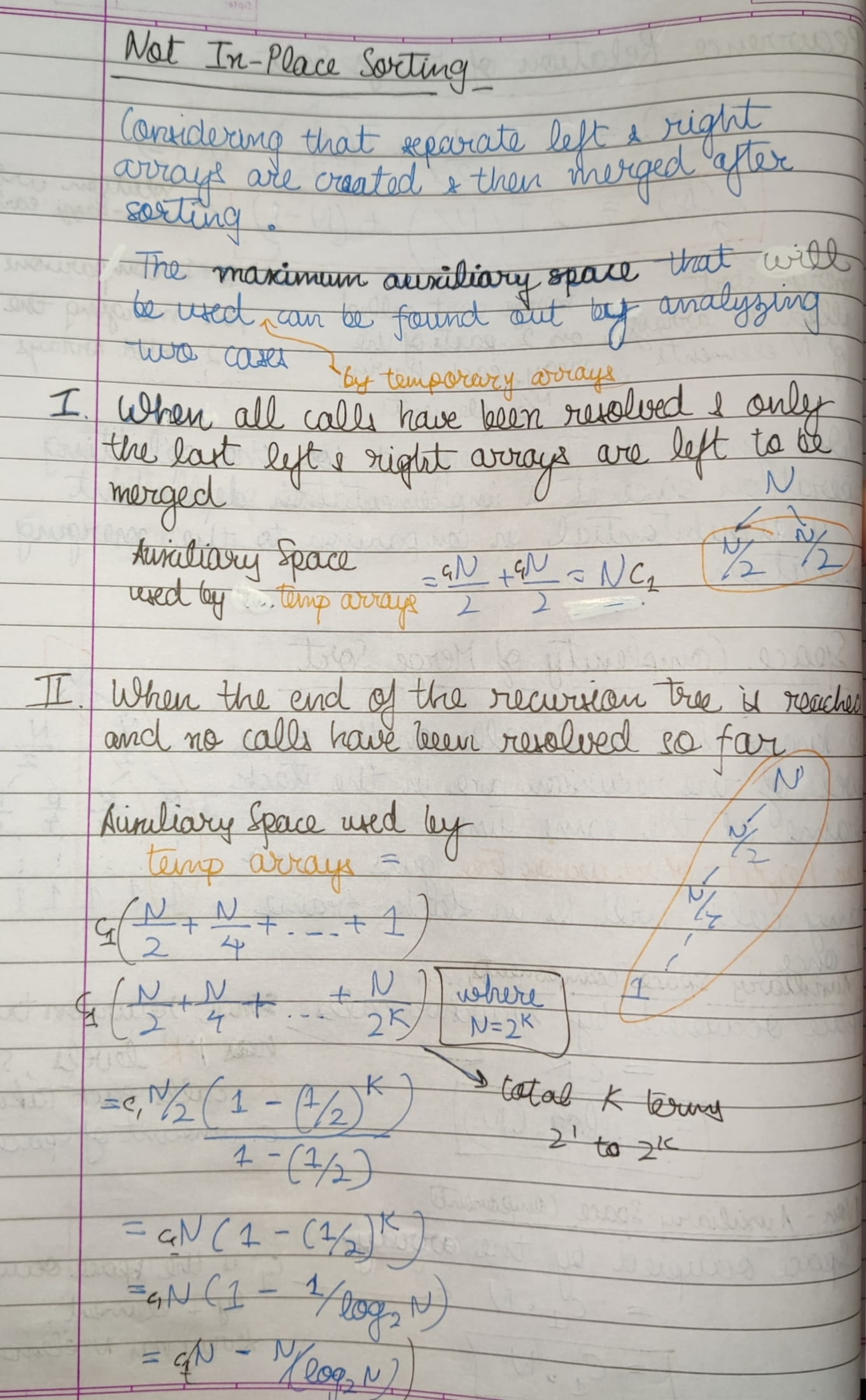
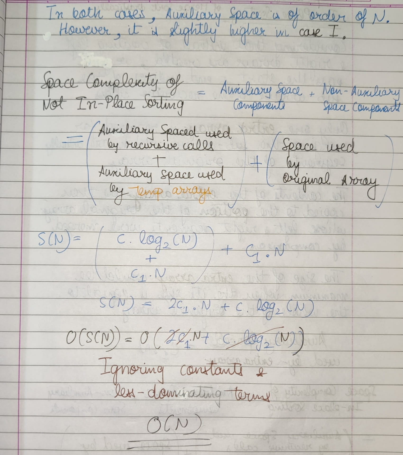
For example, if we want to compare standard sorting algorithms on the basis of space, the auxiliary space would be a better criteria than Space Complexity. Merge Sort uses O(n) auxiliary space, Insertion sort and Heap Sort use O(1) auxiliary space.
Space complexity of all these sorting algorithms is O(n) though.
-
It helps us in solving bigger/complex problems in a simpler way.
-
You can convert recursion solution into iteration and vice versa.
So, solve complex problems using recursion and the convert into recursion to get a more optimized answer.
-
Space complexity is higher. For example, if suppose we print 1000 numbers using recursion, 1000 function calls will go into the stack memory, so space complexity will be O(N).
On the other hand, if we print 1000 numbers using loops, the task will be done in constant space complexity O(1) because only a loop variable will be required for storage and it will be updated with each iteration.
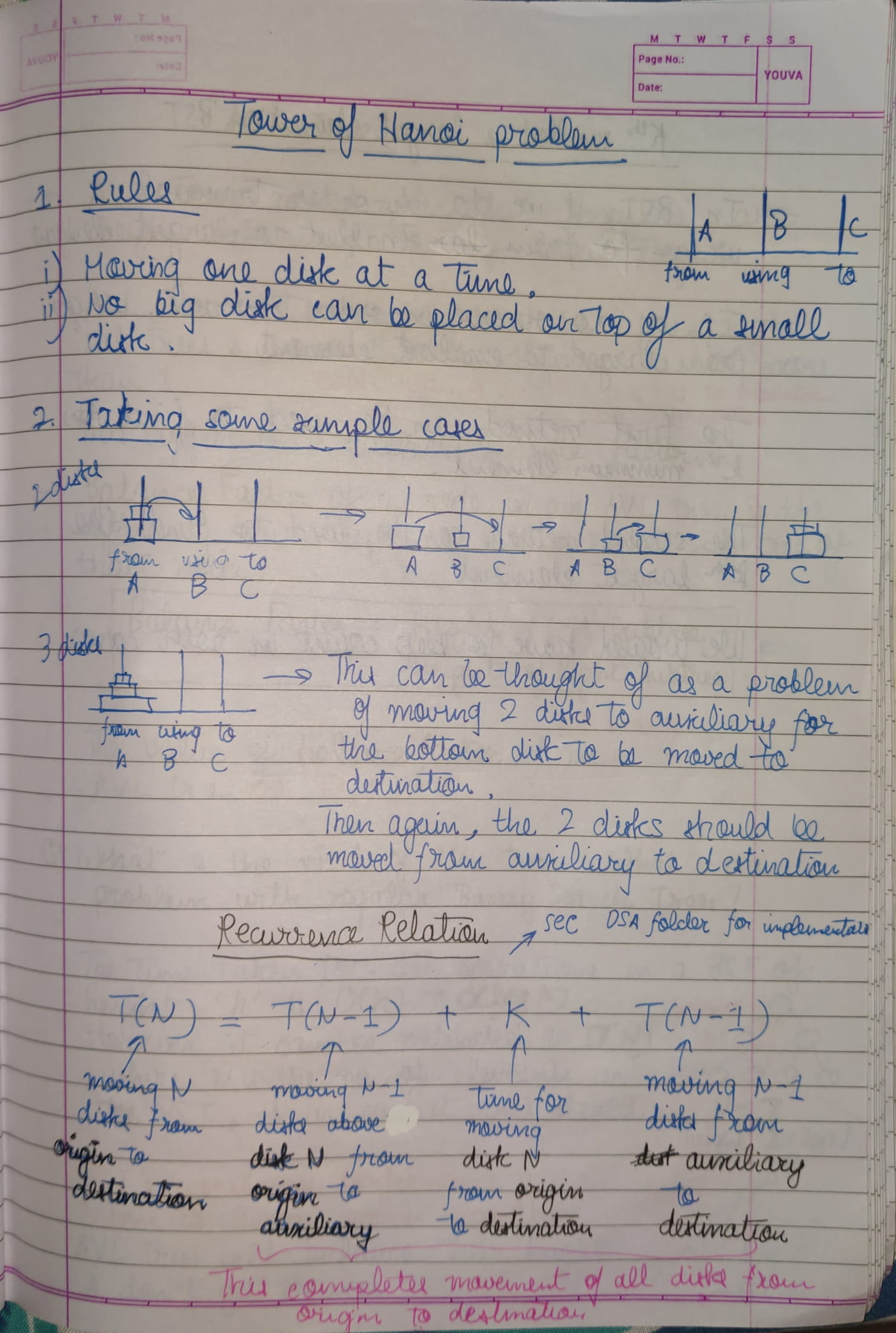
- Identify if you can break down the problem into smaller problems.
- Write down the recurrence relation if needed.
- Draw the recursion tree.
- About the tree:
- See the flow of functions, how they are getting in stack.
- Identify and focus on left tree calls and right tree calls.
- Draw the tree and pointers again & again using pen and paper.
- Use a debugger to see the flow.
- See how and what type of values are returned at each step.
- See at which step, the function call actually finally returns a value.
Why does an error (stack overflow) occur in the case of infinite recursion, when there is no base condition?
Consider the following code snippet:
1  void func() {
2    printf("hello\n");
3    func();
4
5    return;
6  }
7
8  int main() {
9    func();
10 }
In this program, the first function call to func would get stored in the call stack along with the line number of int main at which the control has to be returned after the call to func is over.
Similarly, the internal calls to func will also be stored in the stack frame with the line number 3, which is where the program flow has to continue from once the internal calls to func are over.
This stack memory is not unlimited and after a finite amount of recursive calls, the stack memory would get full; and a stack overflow error would occur.
The recursion tree looks somewhat similar to backtracking because once the base condition is reached, one-by-one the control is returned back up the recursion tree; and finally to the original caller.
Note: Backtracking is performed when:
A viable solution is obtained.
OR
The constraints of the problem we are solving are violated.
The tail recursion is basically using the recursive function as the last statement of the function. So when nothing is left to do after coming back from the recursive call, that is called tail recursion. We will see one example of tail recursion.
For example, if suppose we return (2 + function call), that 2 will be stored somewhere in memory when stack frame of the function, from which the value is being returned, is destroyed.
So instead, we find a way to pass that 2 somehow into the recursive function call.
Factorial calculator using regular recursion:
#include <iostream>

int fact(int n) {
  if (n == 1) {
    return 1;
  };

  return fact(n - 1) * n;
}
In this case, suppose n = 5, the recursive call will make the return value occupy more and more memory until the base condition (n = 1) is reached.
This is how the return value looks with changing n.
( fact(4) * 5 );
( ( fact(3) * 4 ) * 5 );
( ( ( fact(2) * 3 ) * 4 ) * 5 );
( ( ( ( fact(1) * 2 ) * 3 ) * 4 ) * 5 );
( ( ( ( 1 * 2 ) * 3 ) * 4 ) * 5 );
( ( ( 2 * 3 ) * 4 ) * 5 );
( ( 6 * 4 ) * 5 );
( 24 * 5 );
120;
Factorial calculator using tail-end recursion:
#include <iostream>

int fact(int n, int result) {
  if(n == 1) {
    return result;
  }
  return fact(n-1, result * n);
}
In this case, suppose we take n = 5 and a = 1, the return value looks something like this:
fact(5-1,  1 * 5);
fact(4-1,  5 * 4);
fact(3-1, 20 * 3);
fact(2-1, 60 * 2);
120;
Here, as we can see, only the parameters of the function that is getting returned are getting changed, until the base condition (n = 1) is reached. So space complexity in the memory stack is O(1).
While the function is not finished executing, it will remain in stack.
When a function finishes executing, it is removed from the stack and the flow of the program is returned to the point where the function was called.
Fibonacci Recurrence Relation
Fibo(N) = Fibo(N - 1) + Fibo(N - 2)
Here, the argument is getting reduced LINEARLY, which is why it is referred to as Linear Recurrence Relation.
This is quite inefficient because the argument is getting reduced very slowly and at a constant rate. In comparison, in Divide & Conquer Recurrence Relations, division/multiplication by a factor results in exponential change which is much faster and efficient.
Divide-and-conquer algorithms consist of:
- Dividing the problem into smaller sub-problems.
- Solving those sub-problems
- Combining the solutions for those smaller sub-problems to solve the original problem
NOTE that the sub-problems should be of the same type as the main problem.
For example, if the main problem is of SORTING an array, the sub-problem can ONLY be SORTING a part of the array.
Recurrence Relation for Binary Search
Search(N) = O(1) + Search(N/2)
Here, when we try to search for an element using Binary Search, a comparison takes place (in constant time) between the element to be found and the element in the middle of the array, which explains the O(1) term.
After it is determined whether the element to be found is greater or lesser than the middle point, a Search operation is again initiated at either the first or second half of the array, which explains the Search(N/2) term.
Since the search space is DIVIDED by a factor, it is referred to as a Divide & Conquer Recurrence Relation.
As the recursive functions are calling itself again and again, addresses are added into stack. So, if the function is called N times recursively, it will take
Dynamic Programming is a technique in computer programming that helps to efficiently solve a class of problems that have overlapping subproblems and optimal substructure property.
If any problem can be divided into sub-problems, which in turn are divided into smaller sub-problems, and if there are overlapping among these sub-problems, then the solutions to these sub-problems can be saved for future reference.
In this way, efficiency of the CPU can be enhanced. This method of solving a solution is referred to as dynamic programming.
See examples of question solved using dynamic programming under the dynamic-programming directory.
An array is a homogenous data structure: all elements are of the same type. Also, the elements of an array are stored in adjacent memory locations.
Because each cell has the same type (and thus the same size), and because the cells are adjacent in memory, it is possible to quickly calculate the address of any array cell, given the address of the first cell, which is why arrays are good for RANDOM ACCESS of elements.
Say we allocate memory for an array of N elements (the total number of cells of the array must be defined beforehand), where the elements of the array are of a type that has a size of b bytes (e.g. a C++ int has a size of 4 bytes), and the resulting array is allocated starting at memory address x.
Using 0-based indexing:
- the element at index
i = 0is at memory addressx - the element at index
i = 1is at memory addressx + b - the element at index
iis at memory addressx + bi.
Below is the same example array, where the number inside each cell is the index of that cell, and the number below each cell is the memory address at which that cell begins.
An Abstract Data Type specifies:
- Data stored
- Operations on the data
- Error conditions associated with operations
There is no need for contiguous memory like in an array.
Each node consists of 2 things:
- Value stored in node.
- Pointer pointing to memory of next node.
Head of linked list points to the first node.
The last node of the linked list points to a null value.
We define a struct containing an number as well as a pointer to the same struct (Self Referential structure).
We create a pointer of this struct type which is the 'head' pointer of the linked list.
The pointer of the last node is assigned the defined constant NULL, used as an end-marker for the linked list.
NULL is a defined constant that can be implicitly/explicitly type-casted to any pointer type.
It is a pointer that doesn't point to any valid data object.
Considering this code:
#include <iostream>

int main() {
    int* integer = NULL;
    std::cout << integer << std::endl;
    printf("%p", integer);

    return 0;
}
The output of the following code will be:
0
(nil)
It is always a good practice to assign the pointer NULL to a pointer variable in case you do not have exact address to be assigned.
This is done at the time of variable declaration.
A pointer that is assigned NULL is called a null pointer.
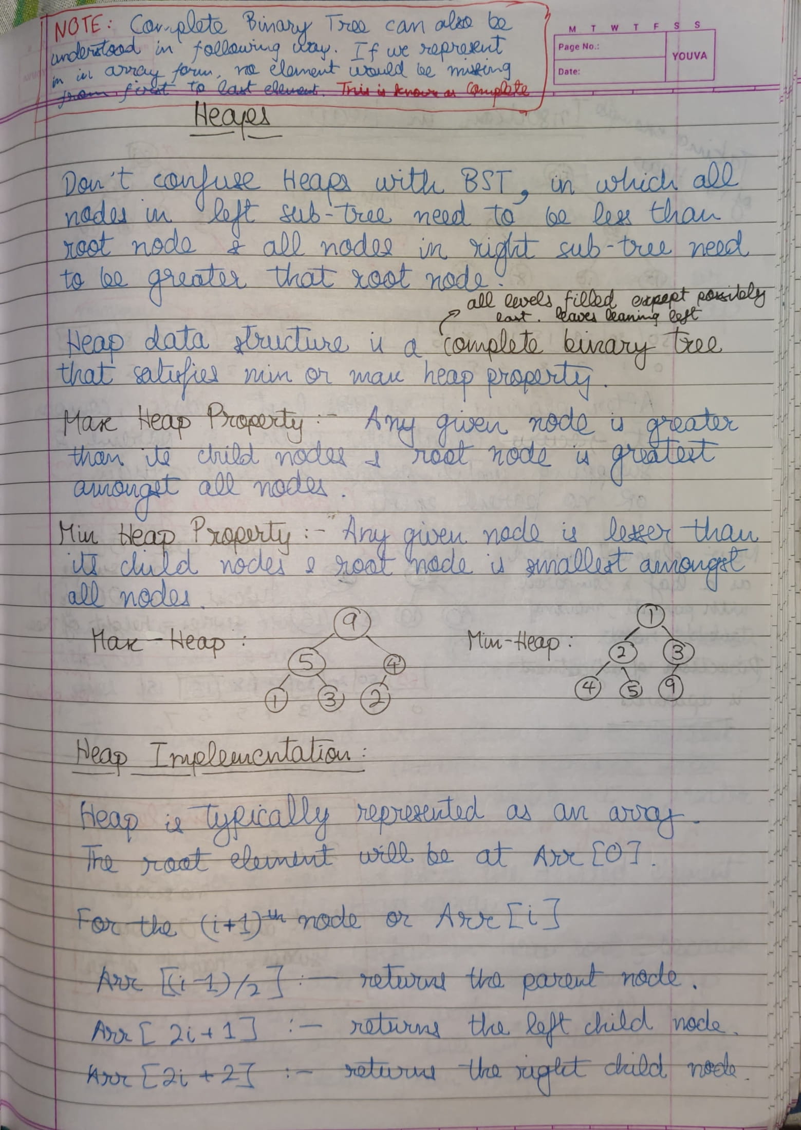
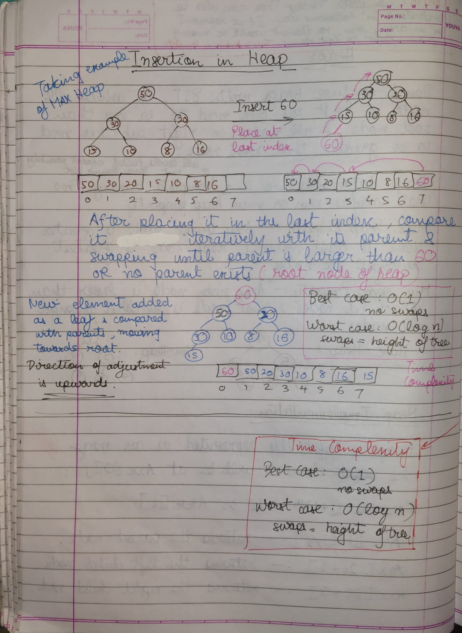
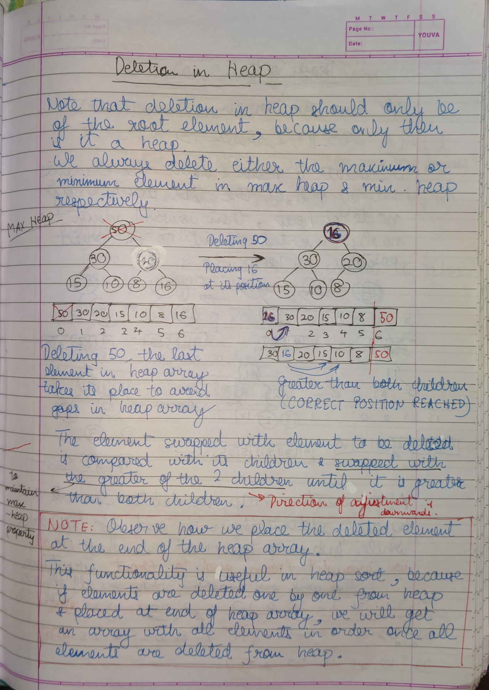
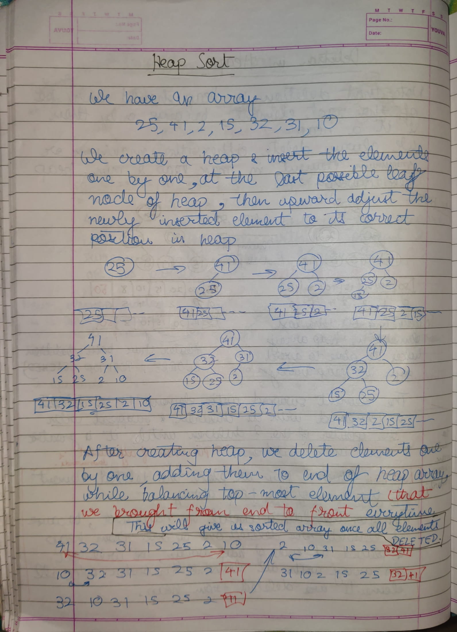
Stack is an ADT that manages data elements linearly but provides access to only one end i.e., data element can be inserted and removed from one end only.
It is a Last-in-First-Out data structure.
It consists of an array whose size is set by the user and can't be changed along with a top pointer to point to the 'top of the stack' or the last filled element.
create()-push()- for adding an element onto the top of the stack.pop()- for deleting an element from the top of stack and returning the element. -1 is returned whenpop()fails.peek()- access the element at the top of the stack.isEmpty()- for checking whether the stack is empty before trying to pop.isFull()- for checking whether the stack is full before trying to add an element.
TODO
We can use stacks to reverse data. (example: files, strings). Very useful for finding palindromes.
It is an algorithmic technique for solving problems recursively by trying to build a solution incrementally, one piece at a time, removing those solutions that fail to satisfy the constraints of the problem at any point in time.
Stacks are used to implement function calls by creating a stack frame in memory where local variables are stored.
As the scopes of the variables end, they are one-by-one popped out from the stack, with the return address at the bottom, after which the stack frame is removed from memory.
Most compilers implement function calls by using a stack.
-
Arithmetic expression evaluation: An important application of stacks is in parsing.
In high level languages, infix notation can't be used to evaluate expressions. A common technique is to convert a infix notation into postfix notation, then evaluating it.
TODO: Understand java bytecode is evaluated on virtual stack based processor
We can start entering elements from the end or the beginning of the array.
We usually implement the top pointer in a simple manner where top is just an integer with a value of the index of topmost element. The value of top is kept as -1 if the stack is empty.
TODO: Stack implementation using Linked List
-
The
frontpointer points to the oldest element in the queue -
The
rearpointer points to the newest element in the queue -
front is actually the first element of the array
-
rear is actually the last element of the array
isEmpty()isFull()enQueue()deQueue()printQueue()
It is opposite to the implementation of stacks using arrays. In stacks, the beginning of the array represented the bottom of the stack for easy pushing and popping.
Here the beginnning of the array is considered as the front of the queue over here.
The implementation of the front and rear pointers is usually kept simple by keeping them as integers storing values of indices.
Initially, front = -1 and rear = -1.
When one element is queued, front is -1 and rear is 0.
Whenever front = rear, queue is empty.
-
Using arrays: Here, enqueueing and dequeueing is an O(1) operation.
But, there can be a case where the queue isn't full, but due to dequeueing, there is extra space at the start of the array.
In this situation, enqueueing an element requires shifting of elements towards the beginning of the array, making enqueueing an O(N) operation.
-
Using linked list: Here, both enqueueing and dequeueing is an O(1).
-
Using other ADTs
A double-ended queue is similar to a Queue ADT with the added functionality of being able to enqueue and dequeue from both ends of the queue.
DE-queues can further be classified into two types:
In restricted INPUT DE-Queue, enqueueing from front is NOT permitted, however dequeueing from end is permitted.
In restricted OUTPUT DE-Queue, dequeueing from end is NOT permitted, however enqueueing from front is permitted.
- Space is not used efficiently.
- The queue may not be full but the rear pointer may reach the end, requiring us to shift elements for enqueueing to take place.
A circular queue is the extended version of a regular queue where the last element is connected to the first element. Thus forming a circle-like structure. The circular queue solves the major limitations of the normal queue, listed above.
Coming to the indexing of the circular queue (the below indexing is based on an array that has space for 5 elements):
Unlike normal queues where initially, front = -1 and rear = -1, and when one element is queued, front is still -1 and rear is 0; in the case of circular queues, both front and rear are equal to the last index in the array.
So initially, front = 4 and rear = 4.
When one element is queued front is still 4 and rear is 0.
In a regular queue, when the queue is full, the front pointer is -1 and rear pointer is 4. So subtracting rear from front give us size which is 5, indicating that the queue is full.
But, in the case of circular queues there are two possible situations when front = rear:
-
Either there are no elements in the circular queue.
-
Or, the circular queue is full.
If suppose after the circular queue is created (
front=rear= 4), 5 elements are enqueued one-by-one, without any dequeueing taking place. At the end of this, thefrontpointer would be 4 and therearpointer would also be 4.So, this leads to confusion whether the circular queue is empty or full.
To solve this confusion, we need an additional member that tells us the number of elements in the circular queue.
This variable is incremented/decremented as elements are enqueued/dequeued.
-
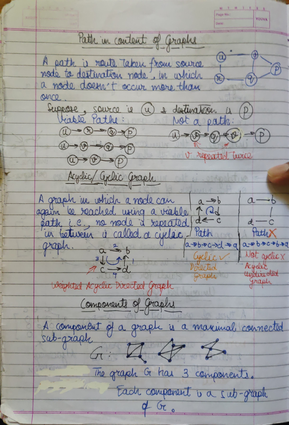
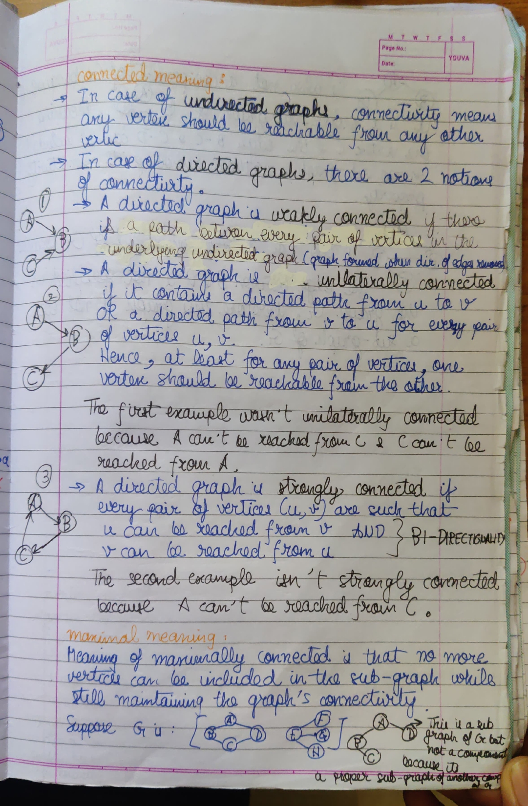
Suppose we have a directed graph with vertices A, B, and C, and directed edges
(A,B)and(B,C).In this case, we would say that A is adjacent to B, B is adjacent to C, but C is not adjacent to B (since there is no directed edge from C to B). Instead, we would say that B is a "successor" of C, or that C is a "predecessor" of B.
-
In an undirected graph, the same set of vertices and edges would be represented as a single undirected edge
(A,B)and another undirected edge(B,C).In this case, we would say that A is adjacent to B, B is adjacent to both A and C, and C is adjacent to B.
This example clarifies the difference between adjacent vertices in directed and undirected graphs.
Once a possible path is found, continue the search until the end of the path.
Start several paths at a time, and advance in each one step at a time
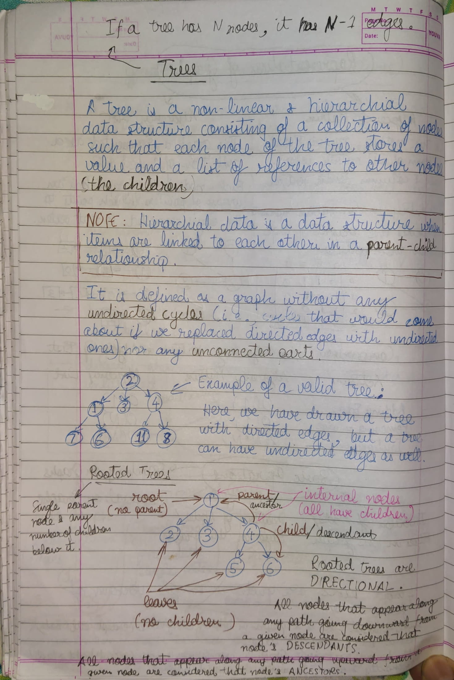
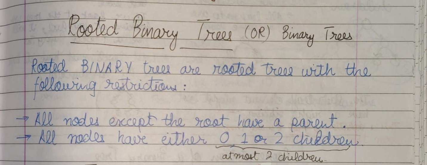
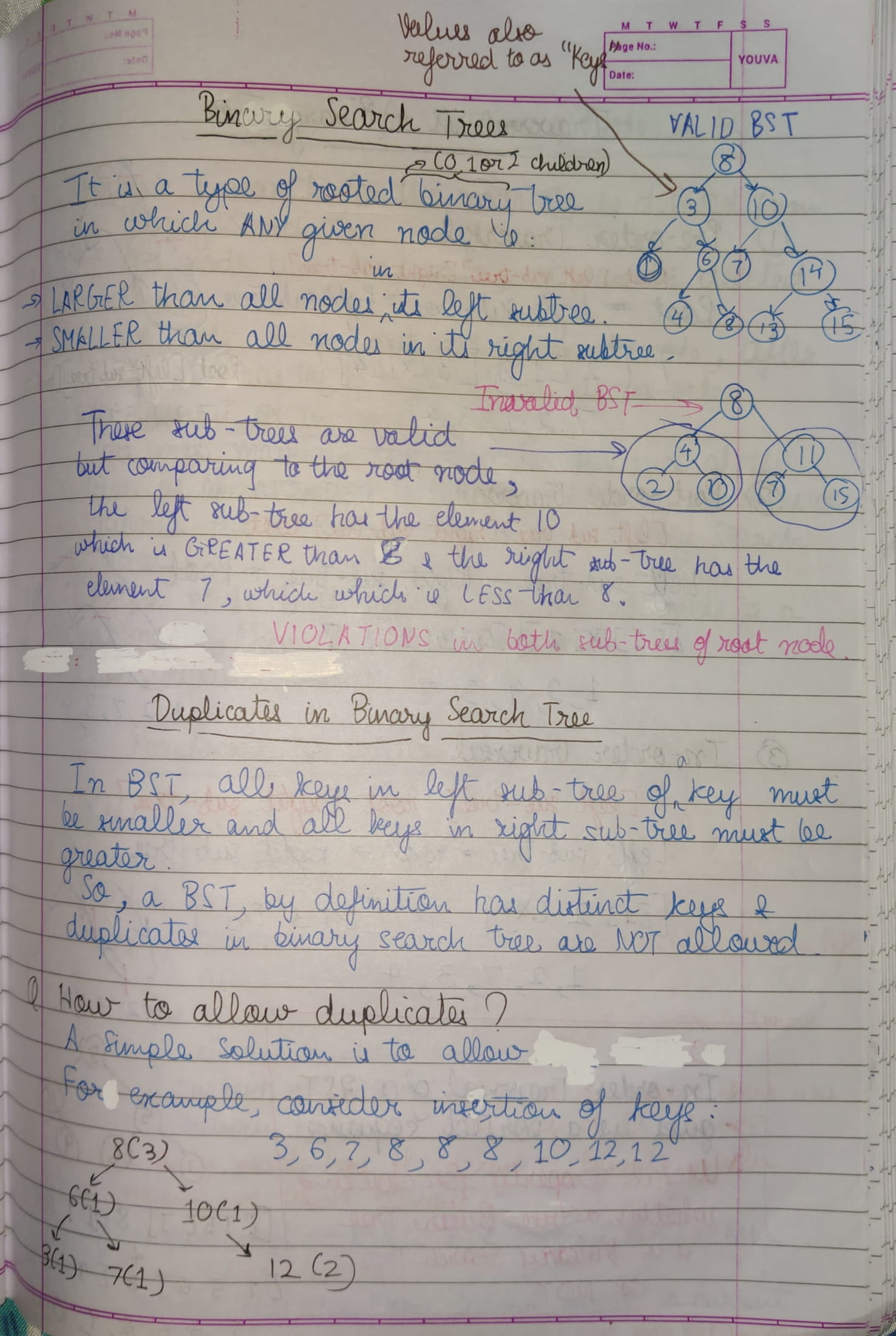
With rooted binary trees (and rooted trees in general), we typically only maintain a pointer to the root because all other nodes in the tree can be accessed via some traversal starting at the root.
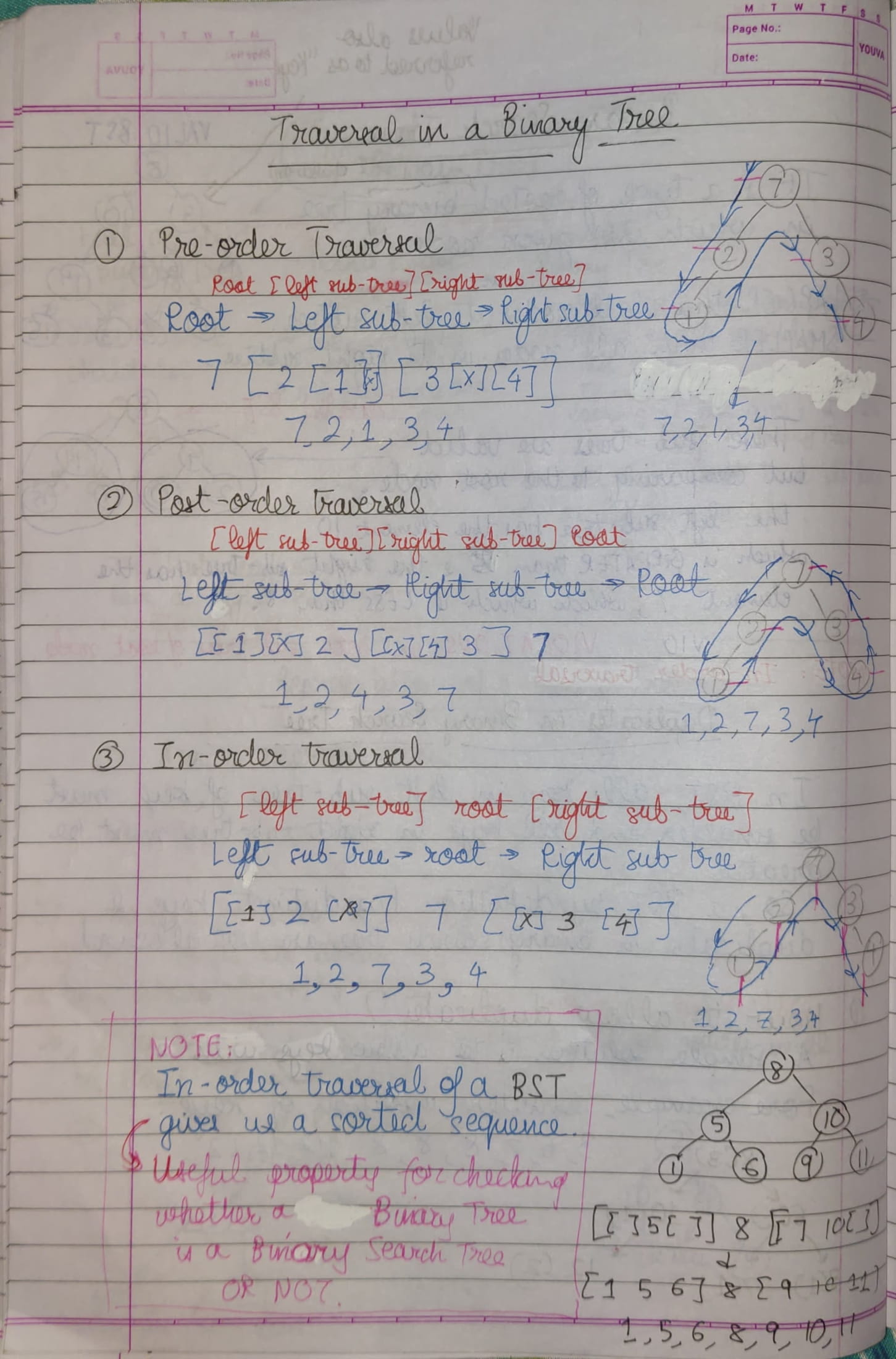
Because we typically only keep track of the root node, to traverse all of the nodes in a rooted binary tree, there are four traversal algorithms:
In all four, the verb "visit" simply denotes whatever action we perform when we are at a given node u (whether it be printing u's label, or modifying u in some way, or incrementing some global count, etc.).
Take the following example of a Tree:
  1
 / \
2   3
   / \
  4   5
- First visit the current node
- Then recurse on the left child (if one exists)
- Then recurse on the right child (if one exists)
Put simply, VLR (Visit-Left-Right).
In the example above, a pre-order traversal starting at the root would visit the nodes in the following order: 1 2 3 4 5
- First recurse on the left child (if one exists)
- Then visit the current node
- Then recurse on the right child (if one exists)
Put simply, LVR (Left-Visit-Right).
In the example above, an in-order traversal starting at the root would visit the nodes in the following order: 2 1 4 3 5
- First recurse on the left child (if one exists)
- Then recurse on the right child (if one exists)
- Then visit the current node
Put simply, LRV (Left-Right-Visit).
In the example above, a post-order traversal starting at the root would visit the nodes in the following order: 2 4 5 3 1
- Visit nodes level-by-level (where the root is the "first level," its children are the "second level," etc.).
- On a given level, visit nodes left-to-right.
In the example above, a level-order traversal starting at the root would visit the nodes in the following order: 1 2 3 4 5
NOTE: This is achievable when Binary Tree is stored as an Array. Printing the array in sequence would give us level-order traversal.
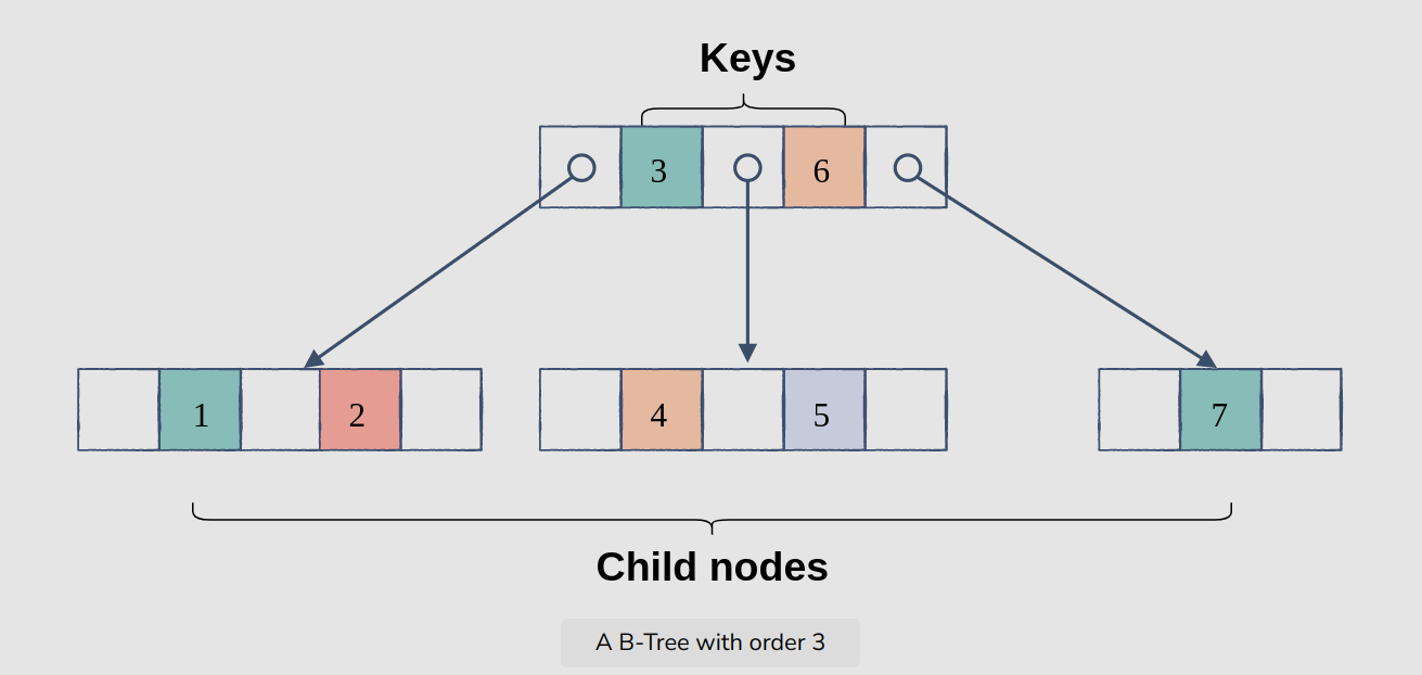
A B-Tree is a self-balancing m-way tree data structure that allows searches, accesses, insertions, and deletions in logarithmic time.
Each node in a B-Tree of order m can have, at most, m children and m-1 keys.
In addition to having multiple children, each node in a B-Tree can have more than one key, which keeps the height of the tree relatively small. This helps with data locality.
In summary, a B-Tree of the order m has the following properties:
- each node has at most m children
- a node with n children must have n-1 keys
- all leaf nodes are at the same level
- every node, except the root, is at least half full
- root has at least two children if it is not a leaf
Read more about it here.
Let us take a case where we wish to store a large amount of data in a tree, that cannot possible fit entirely in our main memory (i.e., RAM) and we would need to use secondary storage devices (e.g., hard disk).
Since the data cannot fit entirely in main memory, it is read from a disk in contiguous chunks or blocks, and written to main memory for processing.
However, reading from a disk is costly as disk access times are far higher than memory access times.
NOTE: Secondary storage devices, like spinnable disks have slower disk access speeds, but have a larger capacity than the main memory (i.e., RAM).
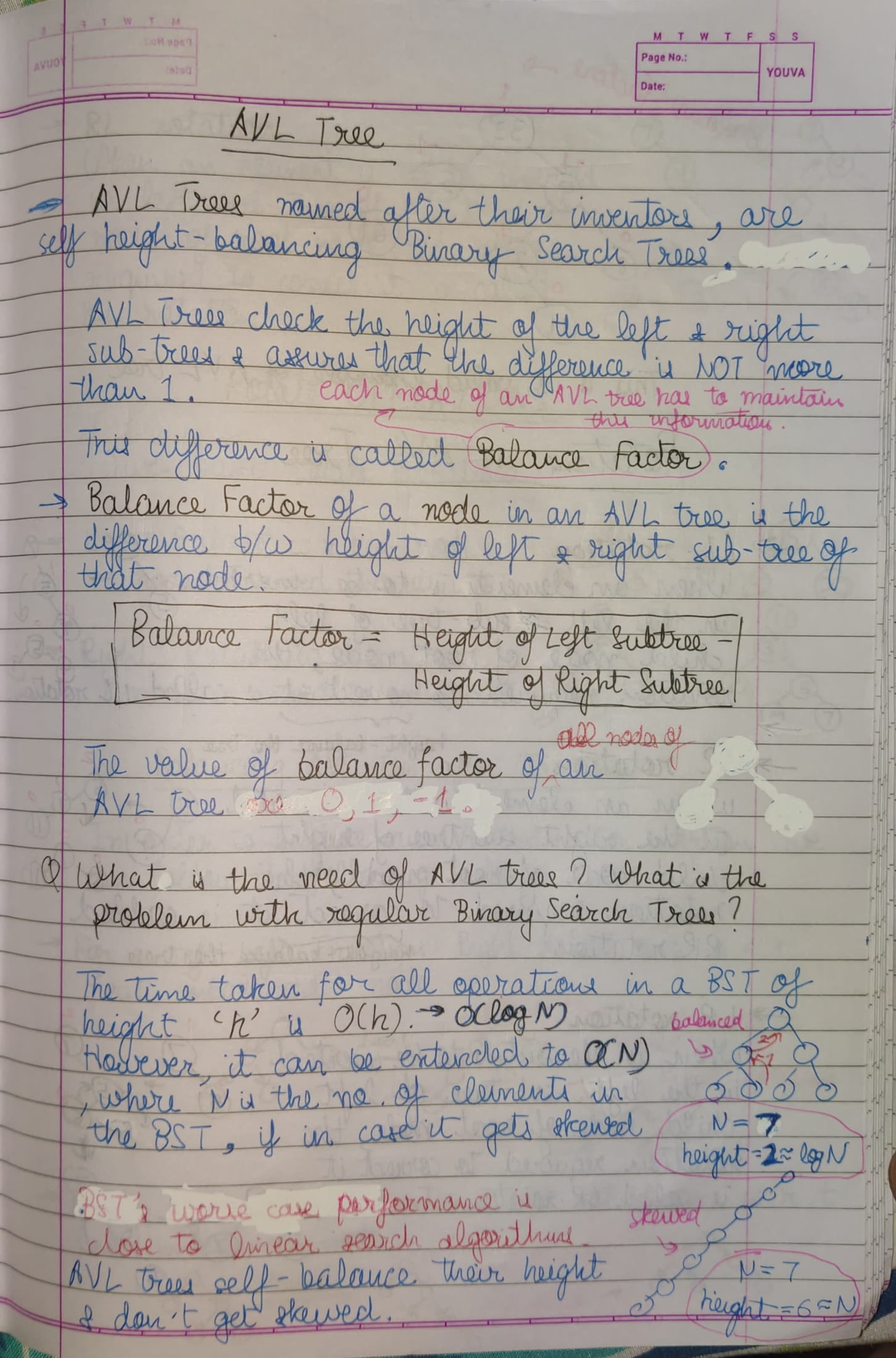
Regular Tree ADTs such as a binary search tree, avl tree, red-black tree, etc can store only one key in one node.
If you have to store a large number of keys, then the height of such trees becomes very large. Due to this, the access time increases because nodes are individually read from memory, one-by-one.
Height of a tree gives us the maximum number of edges from the root node to a leaf. So, in the worst case scenario, for reaching the leaf node of a tree of height h, h disk accesses (dereferencing and accessing each node) would be required.
However, B-tree can store many keys in a single node and can have multiple child nodes.
They also have a high branching factor, meaning the trees are fat with a relatively small height, which ensures minimal disk reads to navigate to the place where the data is stored, for performing its operations, such as insertion and searching.
B-Trees are, therefore, well-suited for storage systems that read and write large blocks of data.
An in-place algorithm is an algorithm that does not need an extra space and produces an output in the same memory that contains the data by transforming the input 'in-place'.
However, a small constant extra space used for variables is allowed.
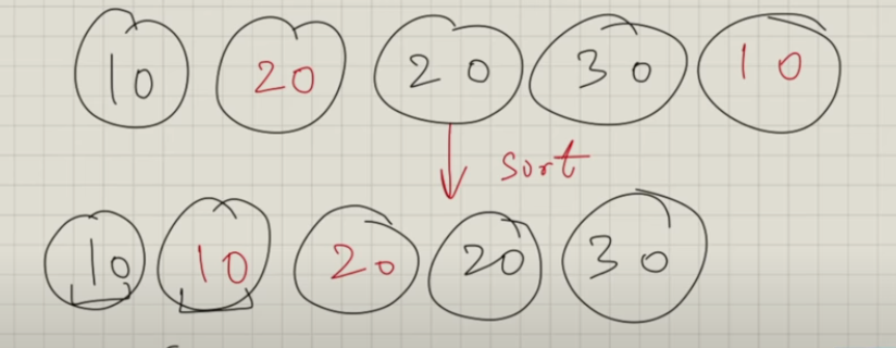
Stable sorting algorithms preserve the relative order of equal elements, while unstable sorting algorithms don't.
In other words, stable sorting maintains the position of two equals elements relative to one another.
An in-place sorting algorithm uses constant space for producing the output (modifies the given array only).
It sorts the list only by modifying the order of the elements within the list.
For example, Insertion Sort and Selection Sort are in-place sorting algorithms as they do not use any additional space for sorting the list.
A typical implementation of Merge Sort is not in-place, also the implementation for counting sort is not an in-place sorting algorithm
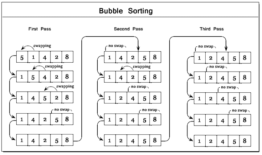
This sorting technique is just like bubbles in a water column, coming up one by one.
In bubble sort, with each subsequent pass, the next largest element is settled at the end of the array.
In each subsequent pass, we reduce our domain of comparison by 1 because 1 additional element is placed in its sorted position after each pass.
It is a stable sorting algorithm as well as an in-place sorting algorithm.
When the array is already sorted, only one pass is run, which includes (N-1) comparisons.
So, it takes minimum amount of time (order of N).
This is implemented using a swap variable which keeps track of how many swaps occur in a single pass.
if(swap == 0) {
    break;
}
else {
    swap = 0;
};- If no swaps occur in a particular pass, then it is clear that the array is already sorted and we need not make any more passes.
- Else, we reset the swap variable for the next pass.
When the array is already sorted, but in reverse order.
The selection sort algorithm sorts an array by repeatedly finding the maximum element (considering ascending order) from unsorted part and putting it at the end.
The algorithm maintains two subarrays in a given array.
- The subarray which is already sorted.
- Remaining subarray which is unsorted.
It is an unstable sorting algorithm as well as an in-place sorting algorithm.
- The good thing about selection sort is that never makes more than (N-1) swaps which is a linear i.e., O(N) complexity, so it can be useful when memory write is a costly operation.
- It performs well for smaller values of N.
The average time complexity is O(N2).
In both the Best and Worst case, all the comparisons will still be made for finding the index position of the next largest element so the time complexity will be almost the same as the average case.
Minor difference can be no time spent in swap operations in the Best Case and all possible swap operations performed in Worst Case.
Insertion sort is a simple sorting algorithm that works similar to the way you sort playing cards in your hands.
The array is virtually split into a sorted and an unsorted part. Values from the unsorted part are gradually inserted place-by-place into the sorted part until they reach their correct position.
After every pass, a larger and larger portion of the array would be sorted.
It is a stable sorting algorithm as well as an in-place sorting algorithm.
- It is adaptive as steps get reduced if array is already sorted.
- It is used for smaller values of N.
- It works well when array is partially sorted.
- It takes part in hybrid sorting algorithms.
When the array is already sorted, only comparison takes place per pass. Number of passes is (N-1) so total comparisons are also (N-1)
So, it takes minimum amount of time (order of N).
When the array is already sorted, but in reverse order.
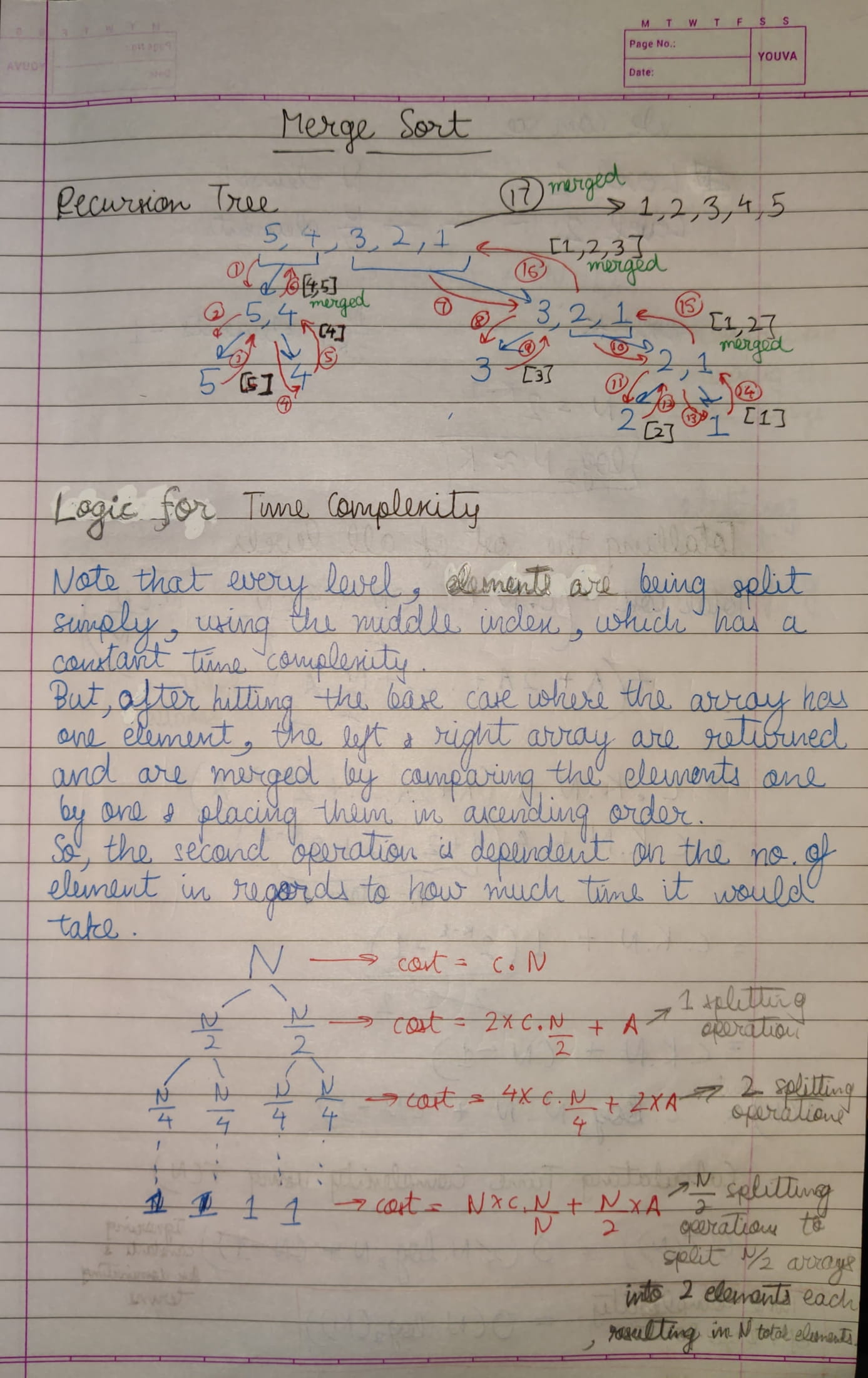
- Divide array into 2 parts
- Get both parts sorted via recursion
- Merge the sorted parts
TODO: correct logic of this
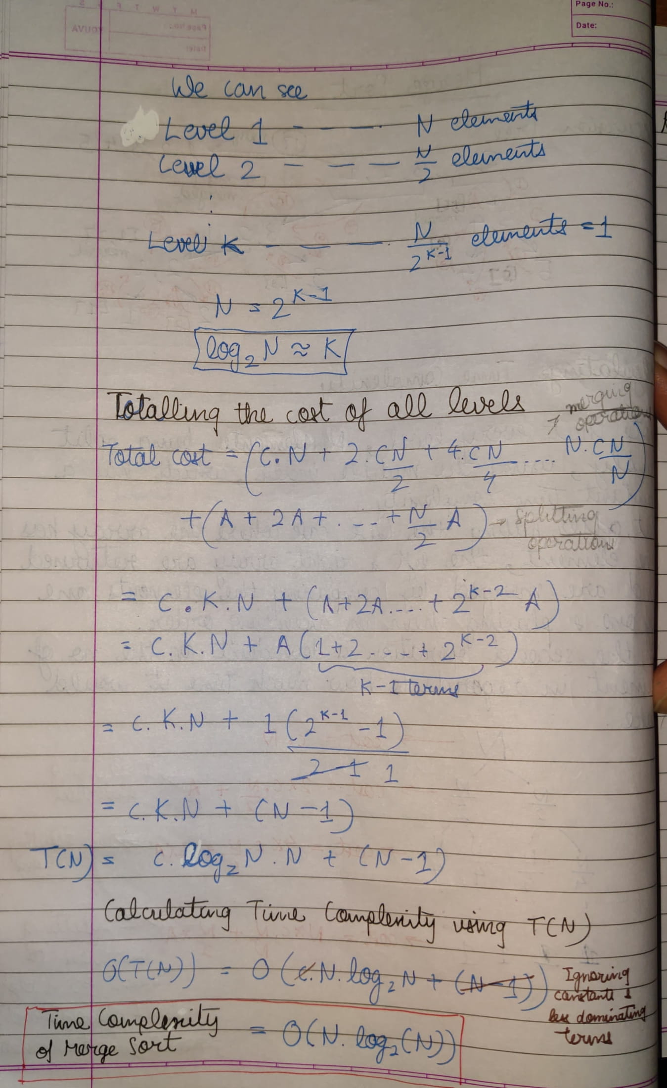
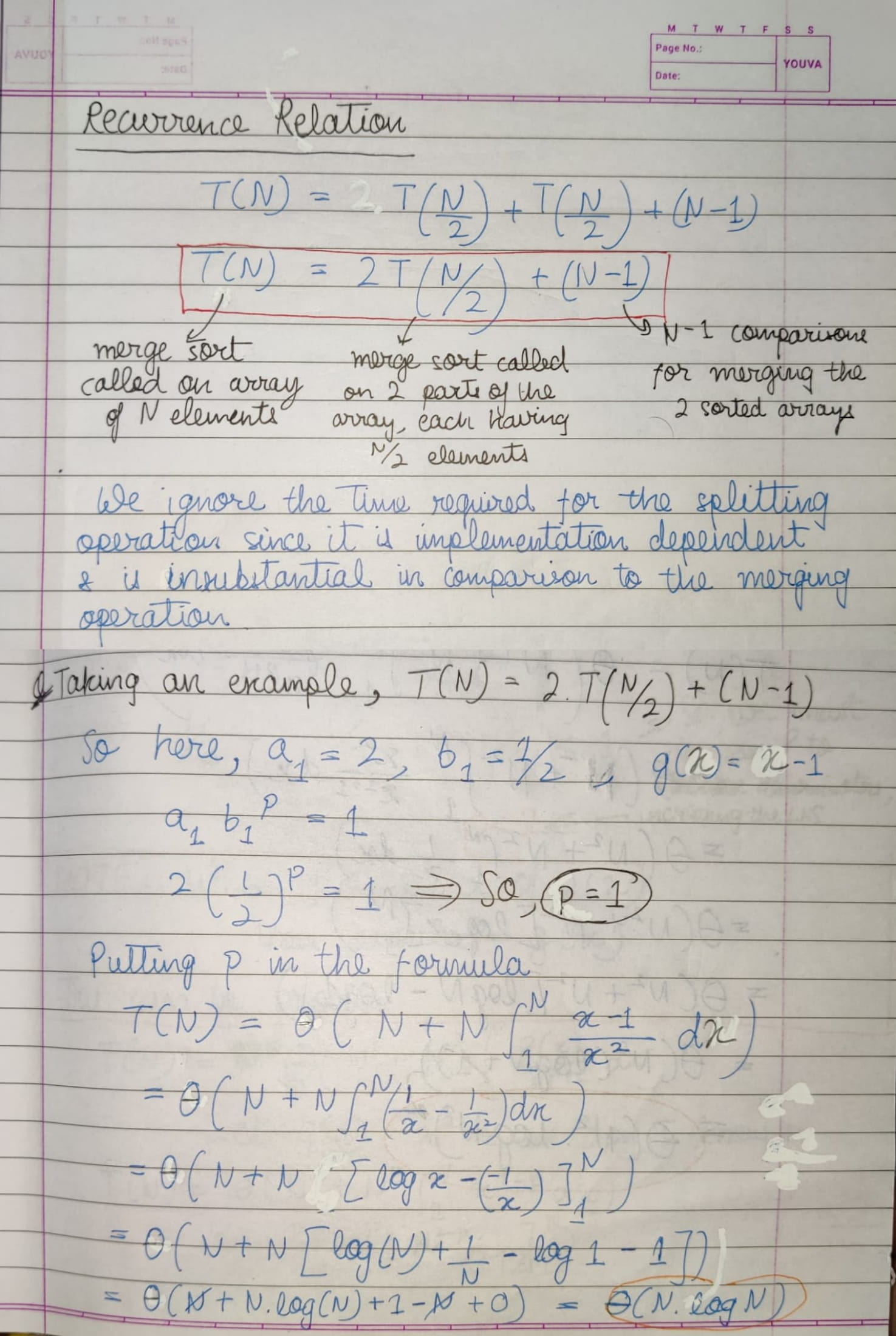
The time complexity of MergeSort is
It is a Divide and Conquer algorithm.
It uses the concept of a pivot for sorting.
It is an unstable sorting algorithm as well as an in-place sorting algorithm.
Quick Sort works by selecting an element called a pivot and placing the pivot element at the correct position after each pass.
Once an element is chosen as a pivot:
- All elements lesser than the pivot will be on the LHS of the pivot.
- All elements greater than the pivot will be on the RHS of the pivot.
It is NOT necessary that the two parts of the array (LHS and RHS of pivot) are sorted. Only the pivot is at its correct position within the array.
There are many different versions of quick sort that pick pivot in different ways.
- Always pick the first element as a pivot.
- Always pick the last element as a pivot (implemented below)
- Pick a random element as a pivot.
- Pick median as the pivot.
We use 4 variables in quick sort:
start: This is the starting index of the partitioned array.end: This is the ending index of the partitioned array.left: This is a dynamic variable used to swap elements which are greater than the pivot, but are present on the LHS of the pivot.right: This is a dynamic variable used to swap elements which are less than the pivot, but are present on the RHS of the pivot.
-
An advantage Quick Sort has over Merge Sort is that if an array is already sorted, Merge Sort will still run till the base condition (the sub-array has only 1 element) is reached, and merge the sub-arrays back to the original array by comparing the elements of the sub-arrays.
Here, that will NOT happen. The only process happening will be incrementation of the left and right pointers.
TODO: How?
-
For arrays, Quick Sort is preferred over Merge Sort, because Merge Sort takes O(N) extra space.
But, in the case of linked lists, memory allocation is random so Merge Sort is preferred over Quick Sort. TODO: Why?
The sorting algorithm used by the in-built sort() method in Python is Tim Sort which is a combination of Merge Sort and Insertion Sort (works well with partially sorted arrays).
TODO : Understand in detail
This is when the target element is found in the very FIRST pass.
This is when the target element is found in the very LAST pass.
TODO
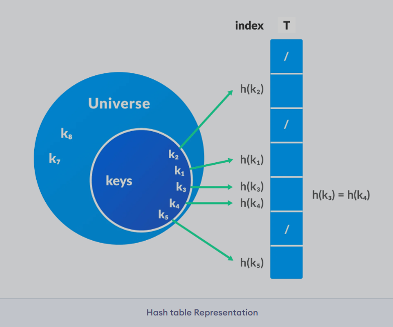
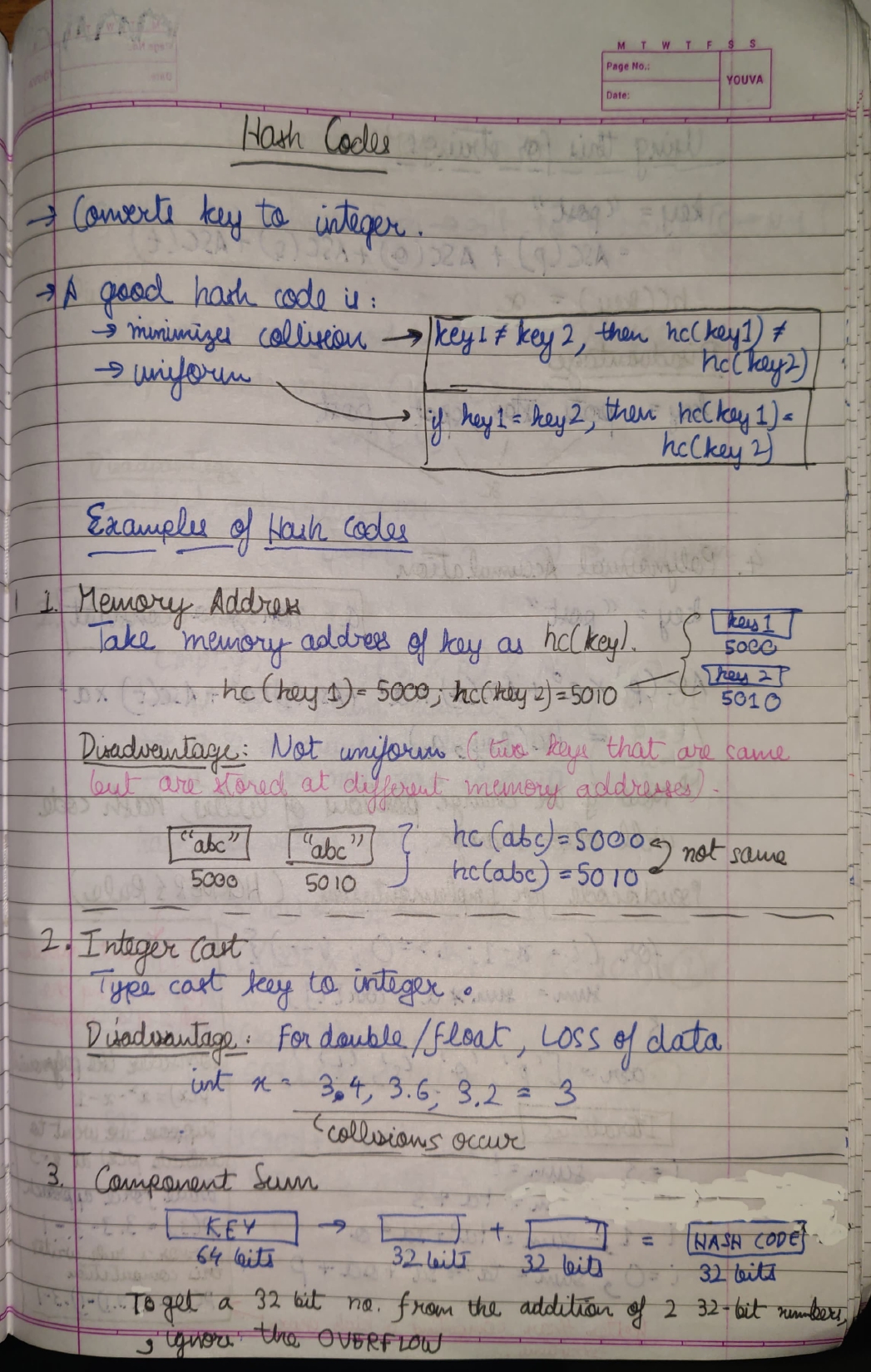
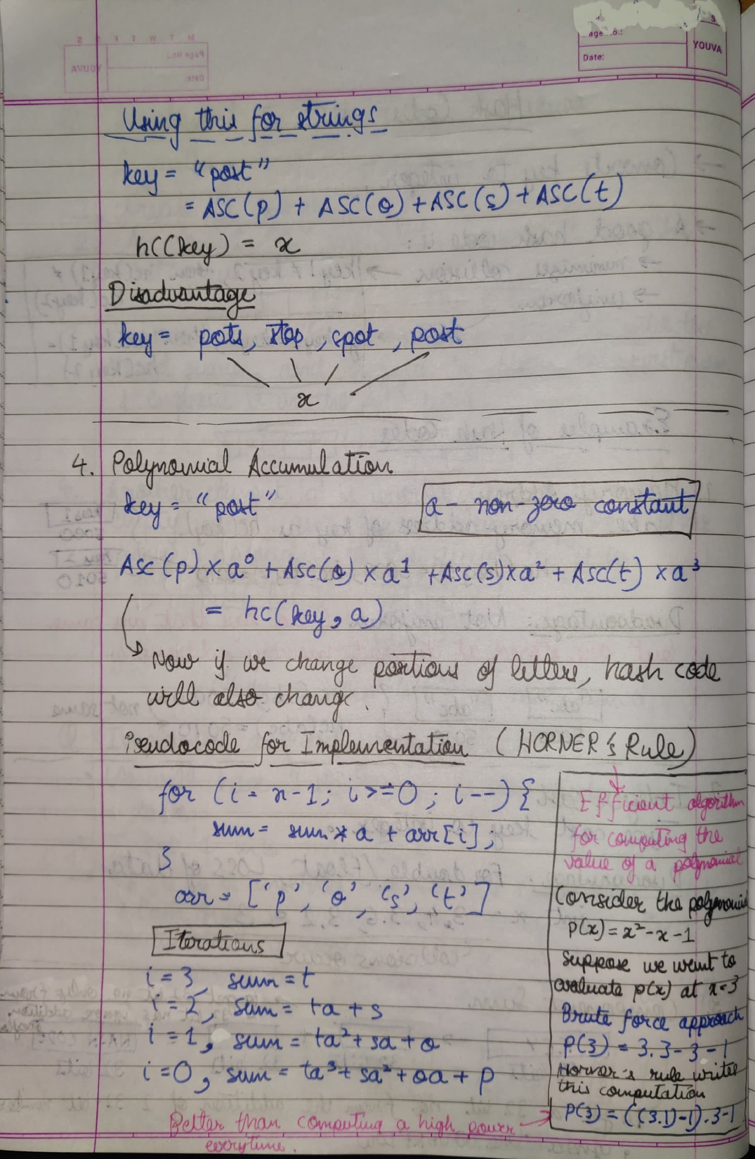
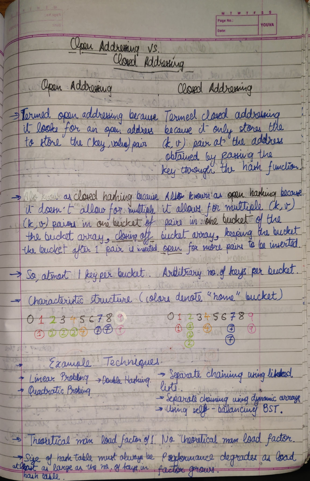
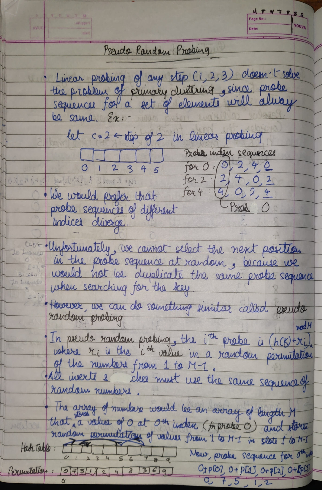
Hashing is the process of converting a given key into another value.
A hash function is used to generate the new value using the key, according to a mathematical algorithm.
The result of a hash function is known as a hash value or simply, a hash.
A good hash function uses a one-way hashing algorithm (the hash cannot be converted back into the original key).
NOTE: It is an ideal method for representing dictionaries for large datasets.
This is because unlike Linear Search and Binary Search, which perform lookups/search with time complexity O(N) and O(log(N)) respectively, Hashing allows lookups in constant time i.e. O(1), since the index-position of the value of a particular key can be figured out using a simple calculation (passing the key into the hashing function, to get the hash value).
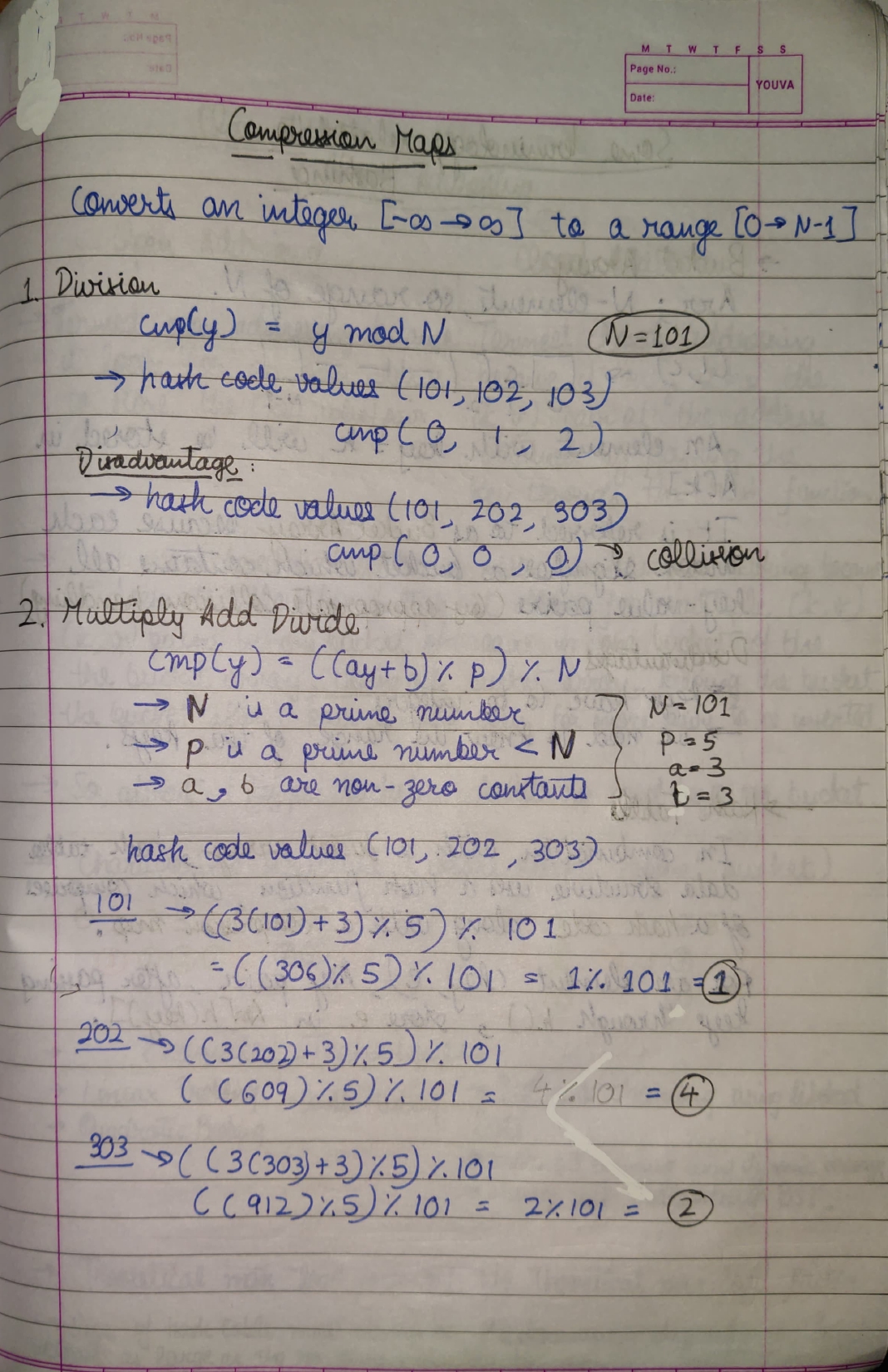
There are two components of any hash function:
- Hash Code: Converts the key (
string,char, object, etc) into an integer. - Compression Map: This part of the function is responsible for getting the hash code (integral value) into the range of the hash table indices. Some examples of these are:
mod10,mod11, etcetera.
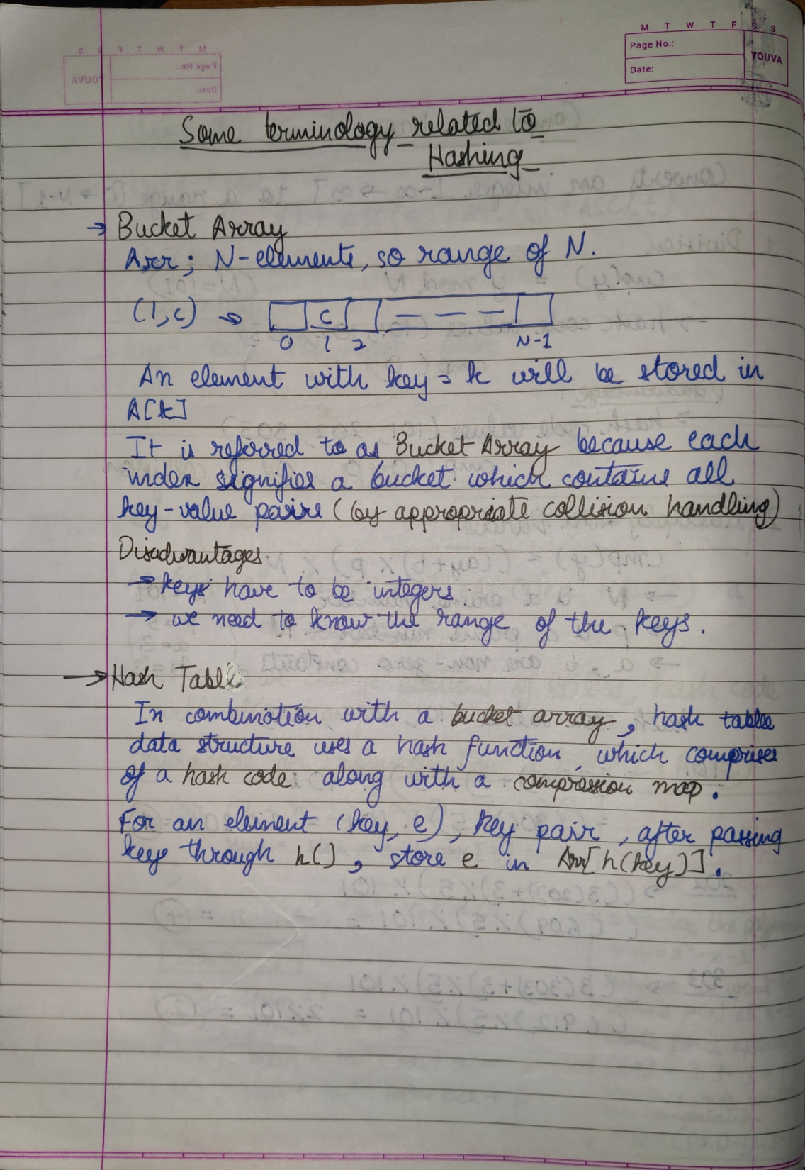
Hash Tables utilize hashing to form a data structure.
In a hash table, hashes obtained by passing keys through hashing functions, are taken as indices.
And, the element corresponding to that key is stored at that index in the hash table.
Considering a key-value pair k, v.
Let k be a key and h(x) be a hash function.
Here, h(k) will give us a new index to store the element v, which is linked with k.
This system of organizing data results in a very fast way to find data efficiently. This is because since each key is mapped to a unique value – once we know a key then we can find the associated value instantly.
In data encryption. Passwords can be stored in the form of their hash so that even if a database is breached, plaintext passwords are NOT accessible.
This is because as mentioned before, good hashing functions don't allow conversion of hash-values back to the original keys, known as pre-image resistance.
Note: Pre-image resistance is the property of a hash function that it is hard to invert, i.e., given an element in the range of a hash function, it should be computationally infeasible to find an input that maps to that element.
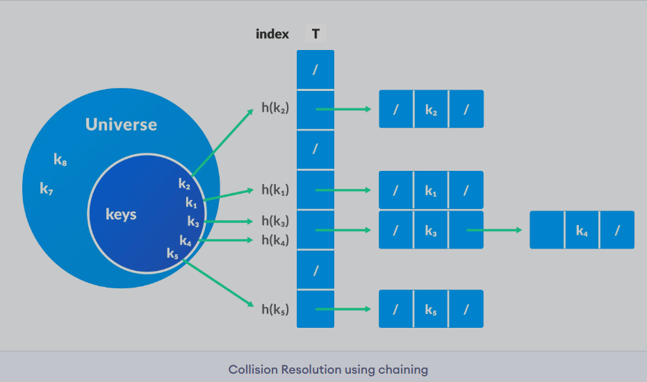
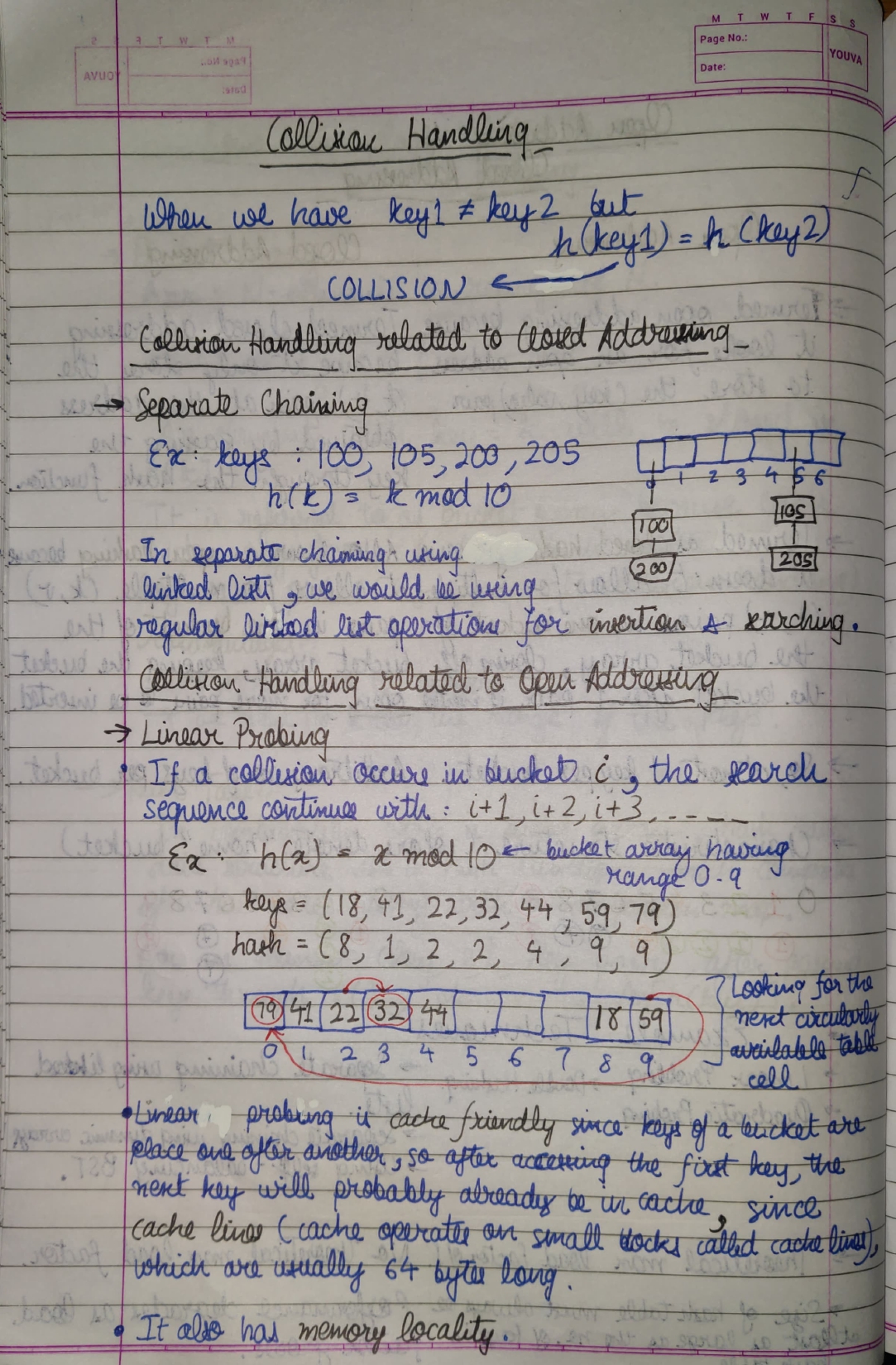
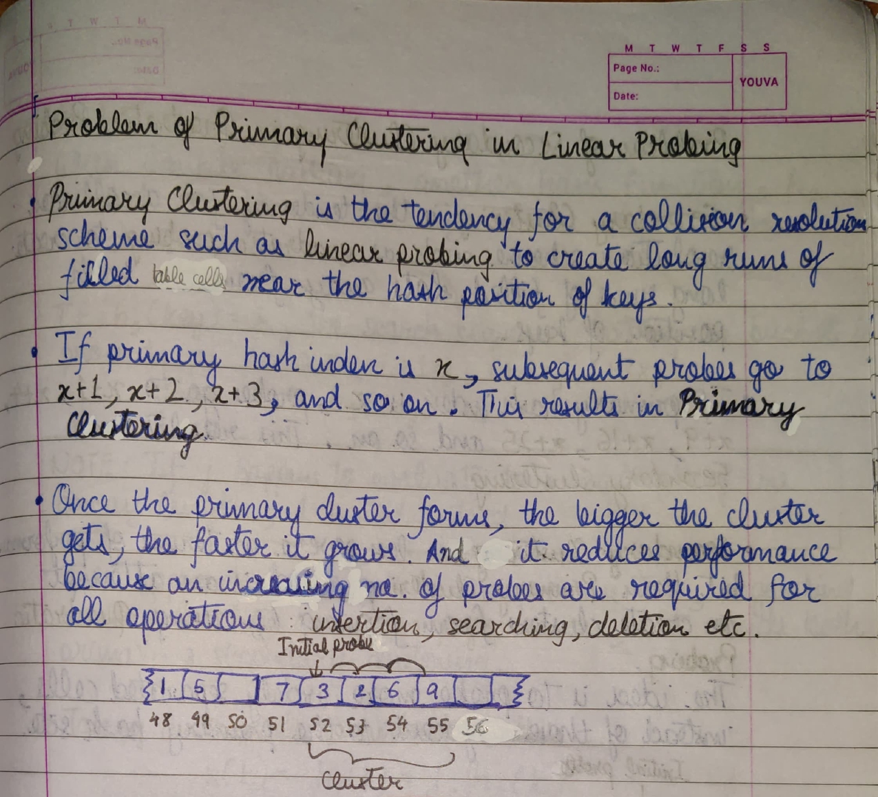
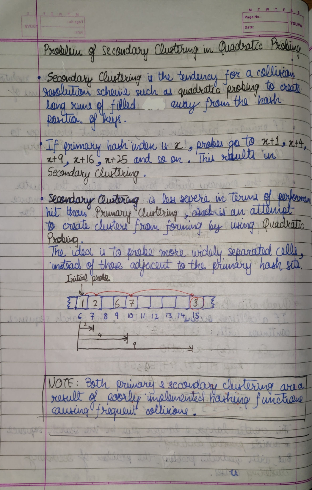
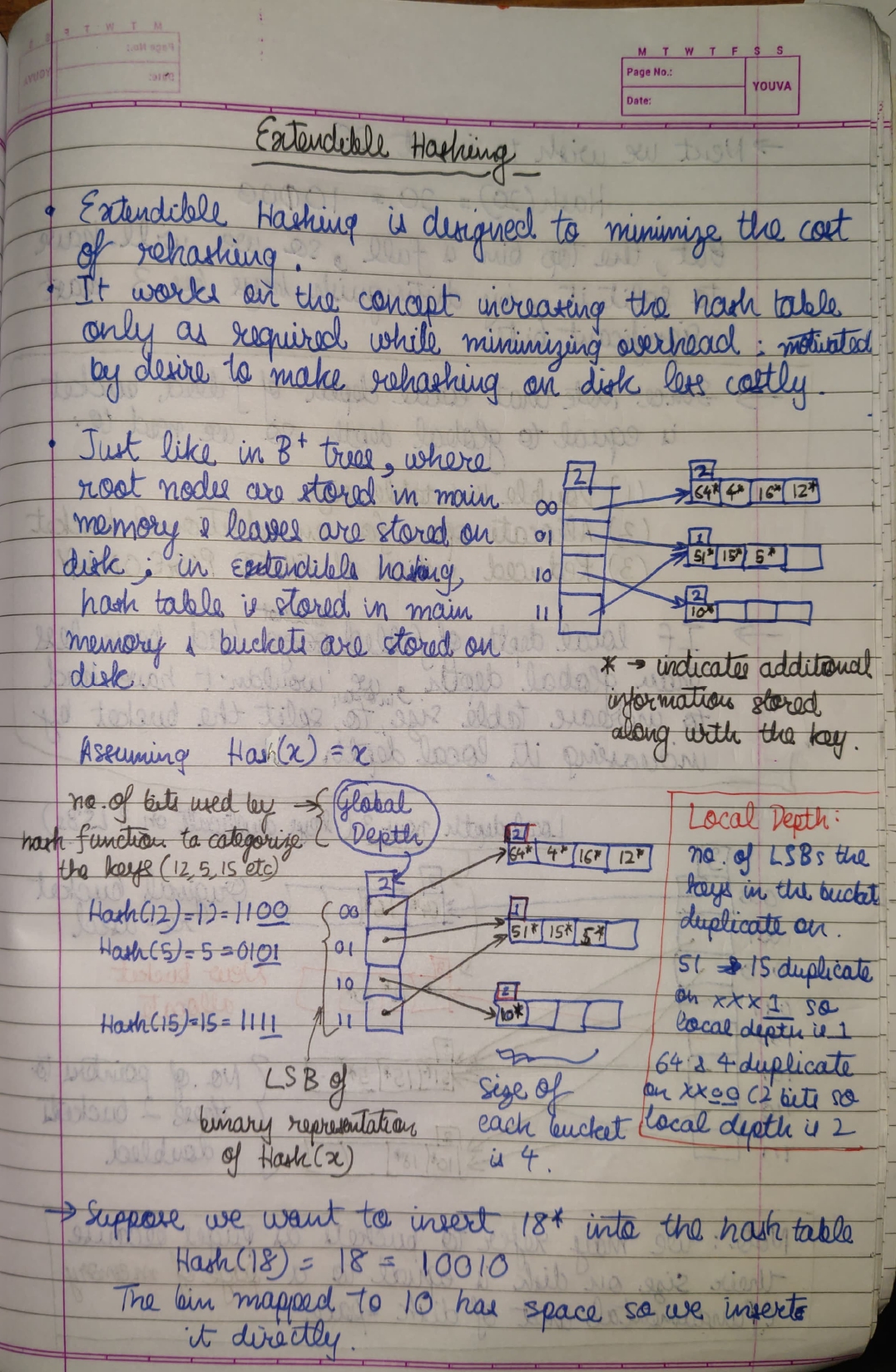
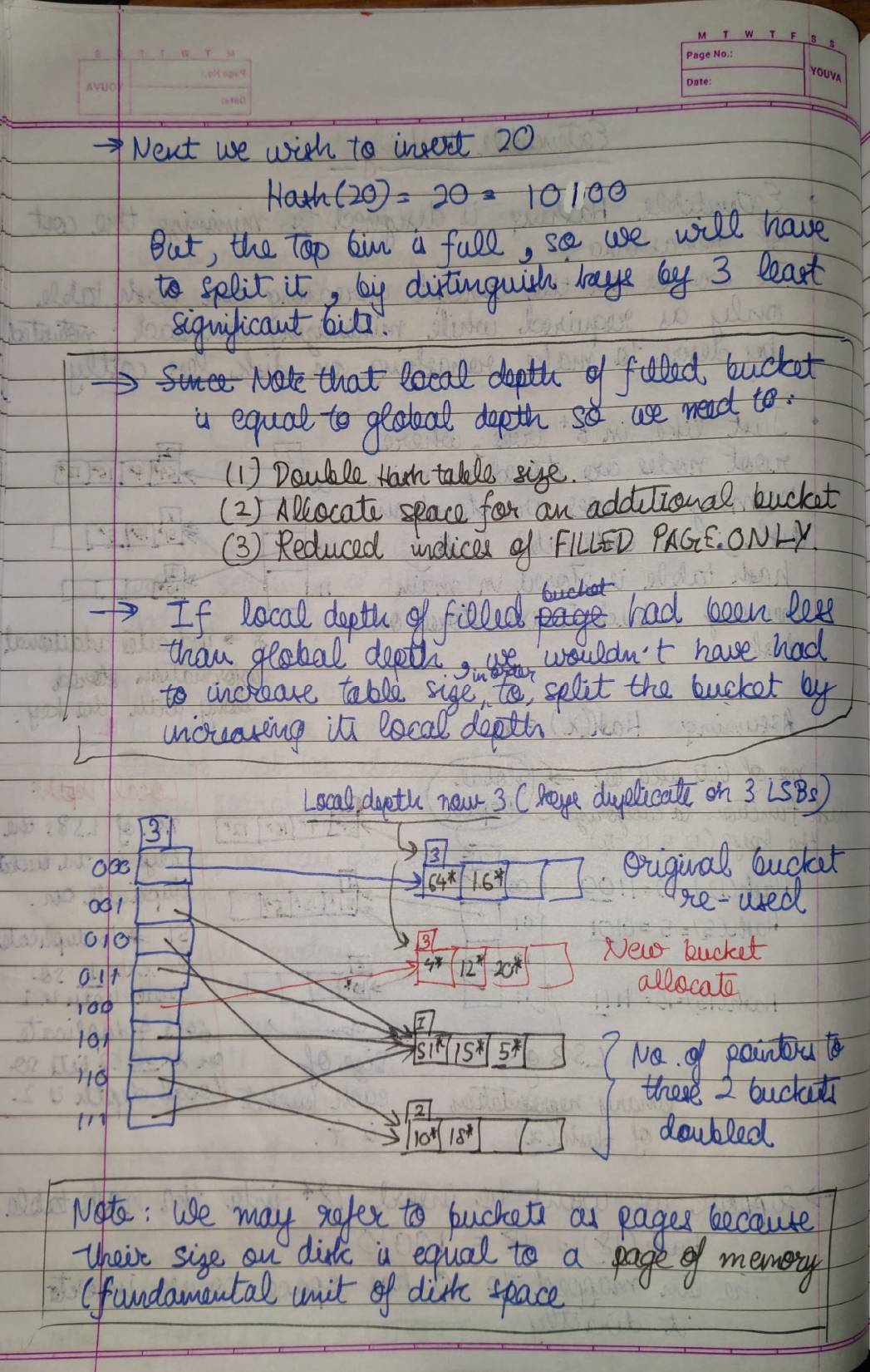
When the hash function generates the same index for multiple keys, there will be a conflict (what value to be stored in that index).
This is called a hash collision.
We can resolve the hash collision using one of the following techniques:
In chaining, if a hash function produces the same index for multiple elements, these elements are stored in the same index by using a doubly-linked list.
If j is the slot/index/hash for multiple elements, it contains a pointer to the head of the list of elements.
If no element is present, j contains NIL.
Read more about on programiz here.
We can make use of the function:
where x is the number whose digits we want to count.
This is because looking at the value of
$\log_{10}1 = 0$ $\log_{10}1 + 1 = 1$
$\log_{10}7 = 0.845...$ $floor( \log_{10}7 ) + 1 = 1$
$\log_{10}10 = 1$ $\log_{10}10 + 1 = 2$
$\log_{10}47 = 1.672...$ $floor( \log_{10}47 ) + 1 = 2$
-
$\log_{10}100 = 2$ , $\log_{10}100 + 1 = 3$
The value of
This is also when an extra digit is added to the number.
So, this is an ideal method for calculating the number of digits of a number.
-
When a loop varaiable is incremented by 1 uptil
$N$ , it runs$N$ times. Looking at an example:for(int i = 1; i <= N; i++) { for(int j = 1, j <= K; j++) { // an operation that takes time `T` } }
-
$(K * T)$ is the time taken by the inner for-loop. - The outer for-loop runs
$N$ times. - Approx. time taken by the outer for-loop in the above case =
$(N * K * T)$
-
-
When it is incremented by
$K$ uptil$N$ , it runs$N/K$ times, approximately. Looking at another example:for(int i = 1; i <= N;) { for(int j = 1, j <= K; j++) { // an operation that takes time `T` } i += K; }
-
$(K * T)$ is the time taken by the inner for-loop. - The outer for-loop runs
$N/K$ times. - Approx. time taken by the outer for-loop in the above case =
$\frac{(N * K * T)}{K}$ =$(N * T)$
-
See the code here.
When we are iterating over the elements of an array, we use incrementation similar to this:
int size = 3;

int index = 0;

while(index < size) {
  int arr[size] = {1, 2, 4};

  printf("%d\n", *(arr + index));

  index++;
}
Here, 0 is incremented to 1, 1 is incremented 2, 2 is incremented to 3.
This would run the while-loop once, since the index variable would reach out of bounds of the indices available in the array arr.
The concept of Circular Incrementation would let this while-loop run infinitely.
Increment operation works in the regular way, 0 is incremented to 1, 1 is incremented 2, BUT 2 is incremented to 0, staying within the index bounds.
The code would look something like this:
int size = 3;

int index = 0;

while(index < size) {
  int arr[size] = {1, 2, 4};

  printf("%d\n", *(arr + index));

  index = (index + 1) % size;
}I mention artifical changing of base because although we seem to have changed the base of the number, we haven't in reality.
The number still has a decimal base.
The only difference it is only using digits of another base, instead of all the decimal digits.
So, if we convert it to base 8, the number will only use the digits 0-7.
-
Integer.toString(int num, int radix)How this method works is, it assumes that
numhas base-10.If we give
radix = 2, it will give us a binary representation ofnumin string form, making the conversion on the assumption thatnumhas base-10. -
Integer.parseInt(int num, int radix)The return value of this function is a integer of base-10.
// Java program to convert one base to other
public class MainClass {

	public static int baseConversion(int number, int toBase)
	{
    /*
    Integer.parseInt using second argument as 10,
    converts the number in `toBase` to normal integer in decimal form.

    The actual value of the integer changes in this process.
    */
		return Integer.parseInt(
		    // Integer.toString converts the decimal number to a string representation in `toBase`
		    Integer.toString(number, toBase), 10
		);
	}

	public static void main(String[] args)
	{
		int number = 955; // Number
		int toBase = 8; // Destination Base Octal

		System.out.println(baseConversion(number, toBase));
	}
}-
Number of Powerful Integers - Leetcode Bi-weekly 121
It can be used to adhere to the limit of the integer.
