Vehicle Detection
The Project
The goals / steps of this project are the following:
- Perform a Histogram of Oriented Gradients (HOG) feature extraction on a labeled training set of images and train a classifier Linear SVM classifier
- Optionally, you can also apply a color transform and append binned color features, as well as histograms of color, to your HOG feature vector.
- Note: for those first two steps don't forget to normalize your features and randomize a selection for training and testing.
- Implement a sliding-window technique and use your trained classifier to search for vehicles in images.
- Run your pipeline on a video stream (start with the test_video.mp4 and later implement on full project_video.mp4) and create a heat map of recurring detections frame by frame to reject outliers and follow detected vehicles.
- Estimate a bounding box for vehicles detected.
Writeup
Histogram of Oriented Gradients (HOG)
1. Explain how (and identify where in your code) you extracted HOG features from the training images.
The code for this step is contained in the in the cells of the IPython notebook under the label HOG Functions.
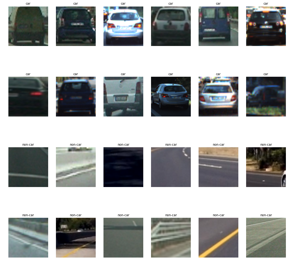
I started by reading in all the vehicle and non-vehicle images. Here are some examples of each of the vehicle and non-vehicle classes:
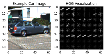
I then explored different color spaces and different skimage.hog() parameters (orientations, pixels_per_cell, and cells_per_block). I grabbed random images from each of the two classes and displayed them to get a feel for what the skimage.hog() output looks like.
Here is an example using the Y channel of the YUV color space and HOG parameters of orientations=9, pixels_per_cell=(8, 8) and cells_per_block=(2, 2):
2. Explain how you settled on your final choice of HOG parameters.
I tried various combinations of parameters using more of a guess and check technique and settled in on the following parameters:
color_space = 'YUV'     # Can be RGB, HSV, LUV, HLS, YUV, YCrCb
orient = 9              # HOG orientations
pix_per_cell = 8        # HOG pixels per cell
cell_per_block = 2      # HOG cells per block
hog_channel = 0         # Can be 0, 1, 2, or "ALL"
spatial_size = (16, 16) # Spatial binning dimensions
hist_bins = 16          # Number of histogram bins
spatial_feat = True     # Spatial features on or off
hist_feat = True        # Histogram features on or off
hog_feat = True         # HOG features on or off
I fiddled with the parameters, extracted the features from the training data, fit a model, ran 10 predictions, and tested the accuracy of the model. The output of those steps was the feedback loop for my process.
For next steps, I'd have liked to do a full factorial sweep on many of the options and looked at the tradeoff between feature extraction time, model prediction time, and model accuracy. There seems to be some clear tradeoffs between these parameters, and there are probably some combinations of model parameters that are better than others.
3. Describe how (and identify where in your code) you trained a classifier using your selected HOG features (and color features if you used them).
The model is trained in the Train the Classifer section of the IPython Notebook.
I used the process outlined in the lectures and quizzes to train a LinearSVC model from the sklearn support vector machine package. The training process involved extracting all of the feature vectors for each image in the car and non-car training images. Because I used both HOG and color features for my model, I normalized the features using this code:
X_scaler = StandardScaler().fit(X)
scaled_X = X_scaler.transform(X)
I then randomly split this data into a test and train set using the train_test_split from the sklearn.model_selection package. The training set was used to train the model, while the test set was used to test the accuracy of the model. Here's what that code looks like:
rand_state = np.random.randint(0, 100)
X_train, X_test, y_train, y_test = train_test_split(
    scaled_X, y, test_size=0.2, random_state=rand_state)
I finally use this data to train the model like so:
svc = LinearSVC()
svc.fit(X_train, y_train)
Sliding Window Search
1. Describe how (and identify where in your code) you implemented a sliding window search. How did you decide what scales to search and how much to overlap windows?
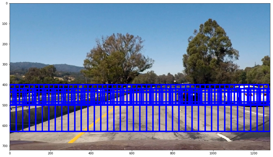
I implement the sliding window search in the section called Find Cars Function. This function is adapted from the same named function from the class work, where it takes in the ystart and ystop values and creates windows in that area. It adds all the windows to a list that produce a match to our car image model. Here's an example of the search area in my algorithm:
Here are the values for the window searching I am using:
| Y Start | Y Stop | Scale |
|---|---|---|
| 400 | 500 | 1.0 |
| 420 | 500 | 1.5 |
| 500 | 650 | 2.0 |
2. Show some examples of test images to demonstrate how your pipeline is working. What did you do to optimize the performance of your classifier?
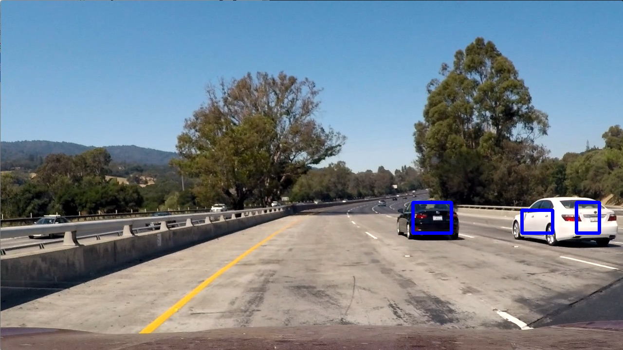
I ran the same set of parameters on the feature extraction for vehicle detection as I used to train my model. I was able to get good results with this number of rectangles, but I found that there is a tradeoff between finding enough rectangles and keeping the search area small to keep the algorithm performant. This seemed to be a decent tradeoff. Here are some of my results:
Video Implementation
1. Provide a link to your final video output. Your pipeline should perform reasonably well on the entire project video (somewhat wobbly or unstable bounding boxes are ok as long as you are identifying the vehicles most of the time with minimal false positives.)
Here's a link to my video result
2. Describe how (and identify where in your code) you implemented some kind of filter for false positives and some method for combining overlapping bounding boxes.
This code lives in the Heatmapping section of the notebook.
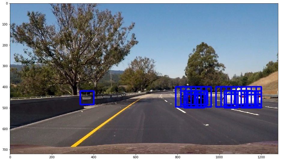
The find_cars() function mentioned earlier produces a set of rectangular boxes where the model says that there are car images. Here's what the outupt of that function looks like, showing all the rectangles that detected vehicles:
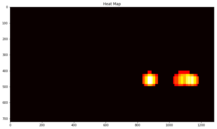
From these positive detection rectangles, I created a heatmap by adding 1 to a binary image where there was a rectangle with this code:
heatmap[box[0][1]:box[1][1], box[0][0]:box[1][0]] += 1I then thresholded that map by throwing out all the heatmap areas that didn't have more than 3 positive detections using this code:
heatmap[heatmap <= threshold] = 0Here's what that heatmap looks like:
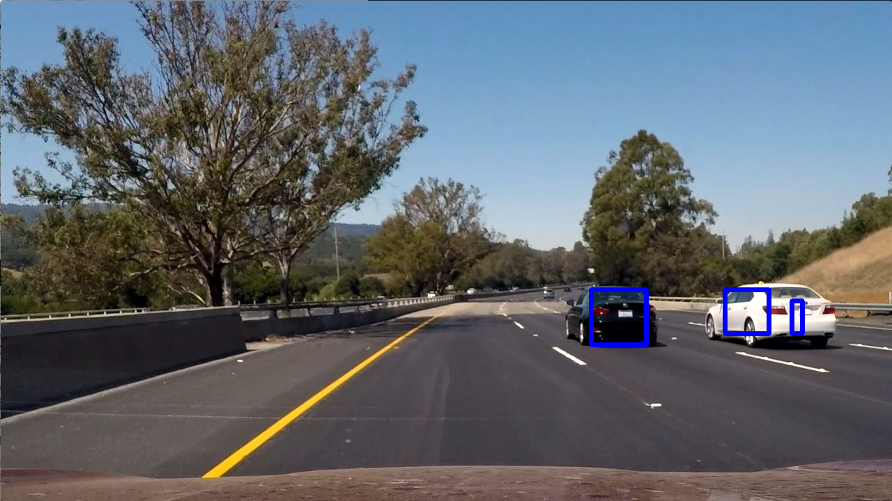
Once I had my vehicle detection areas, I used scipy.ndimage.measurements.label() to identify individual blobs in the heatmap and assumed that each one belongs to a vehicle. I constructed bounding boxes to cover the area of each blob detected.
Here's what the final output looks like:
In addition to these methods, I also use a deque structure to keep track of the previous 5 heatmaps when processing a video. I add these previous heatmaps together with the latest one and apply the same threshold times the number of heatmaps I've added together. This system should help get rid of unwanted detections because if there is only one frame that detects an outlier, then the odds are reduced that we will categorize that detection as a vehicle since it only happened in one frame.
Discussion
1. Briefly discuss any problems / issues you faced in your implementation of this project. Where will your pipeline likely fail? What could you do to make it more robust?
The biggest problem I encountered is lack of performance with the pipeline. I need to make things a lot faster if I want it to run in (near) real time. I could reduce the number of features that I extract, or try to use even fewer search rectangles for the pipeline. In addition to the speed, my model seems to be pretty sensitive to non-car images. I had to bump up the threshold in the heatmap to eliminate them, but perhaps that's an issue with my model parameter selection.
Here are links to the labeled data for vehicle and non-vehicle examples to train your classifier. These example images come from a combination of the GTI vehicle image database, the KITTI vision benchmark suite, and examples extracted from the project video itself. You are welcome and encouraged to take advantage of the recently released Udacity labeled dataset to augment your training data.
