QOSF Task 2

My attempt at a solution for Task 2 of the screening process for QOSF's mentorship program.

Problem

Implement a circuit that returns |01> and |10> with equal probability.

Requirements :

The circuit should consist only of CNOTs, RXs and RYs.
Start from all parameters in parametric gates being equal to 0 or randomly chosen.
You should find the right set of parameters using gradient descent (you can use more advanced optimization methods if you like).
Simulations must be done with sampling (i.e. a limited number of measurements per iteration) and noise.

Compare the results for different numbers of measurements: 1, 10, 100, 1000.

Solution

Theory

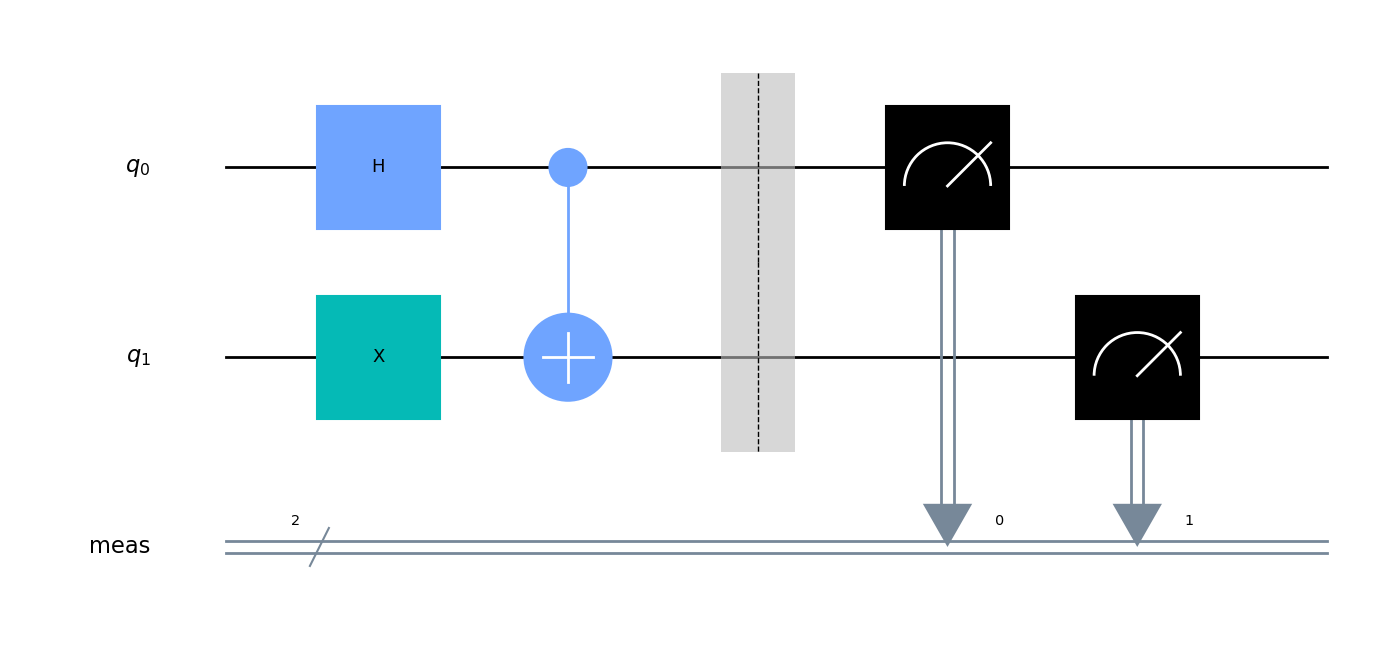
The actual problem statement requires us to use sampling to figure out the parameters, but we may be able to analyze this theoretically to guide us in our search for an appropriate ansatz. Starting from a vector of |0> qubits, we would like to generate |01> + |10>. Below is the simplest way to do this:

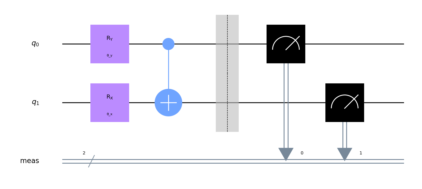
We can replace H = Ry(pi/2) and X = Rx(pi) to meet the gate constraints provided (up to a global phase). All in all, this suggests the following ansatz:

There are some degeneracies for which values of theta give the correct probability distribution, but we expect theta_y to be some half-integer of pi, and theta_x to be some odd integer of pi.

Experiment

Now that we have the ansatz, we can use Qiskit to find the actual parameters. The Qiskit textbook¹ suggests SPSA for simulations with noise, so we'll use that. Qiskit also ships with noise models derived from various IBMQ computers, so we randomly pick one derived from the IBM VIgo here.

    # Get noise model
    vigo_backend = FakeVigo()
    self.noise_model = NoiseModel.from_backend(vigo_backend)
    self.coupling_map = vigo_backend.configuration().coupling_map
    self.basis_gates = self.noise_model.basis_gates

Our goal is to create a circuit that generates |01> and |10> with equal probability, so our cost function should reflect this. Here we use the sum of absolute values of errors between the expected and actual probabilities.

    target_pd = {
            "00": 0,
            "01": 0.5,
            "10": 0.5,
            "11": 0
    }
    
    cost = np.sum([np.abs(observed_pd[k] - target_pd[k]) for k in Task2.POSSIBLE_OUTCOMES])

Results

The script outputs parameters for values of M=[1, 10, 100, 1000], where M is the number of measurements per iteration.

Running test: M=1
====================
Params:
    theta_y: 2.3101941359247484 ( 0.7353576324686674 * pi )
    theta_x: -0.308720184071524 ( -0.09826868665444571 * pi )

Running test: M=10
====================
Params:
    theta_y: 1.5957458026784974 ( 0.5079416648288542 * pi )
    theta_x: 2.8271051395144537 ( 0.8998955151884555 * pi )

Running test: M=100
====================
Params:
    theta_y: 1.595947012571713 ( 0.5080057119270627 * pi )
    theta_x: 3.226977050585924 ( 1.0271786976897102 * pi )

Running test: M=1000
====================
Params:
    theta_y: 1.5621648683948892 ( 0.49725252145909354 * pi )
    theta_x: 3.220890587616747 ( 1.0252413163547294 * pi )

Remember that we expect half-integer multiples of pi for theta_y and odd integer values of pi for theta_x. In this regard, M=1 fares poorly, with results getting better with higher M values (at M=100 we start seeing diminishing returns).

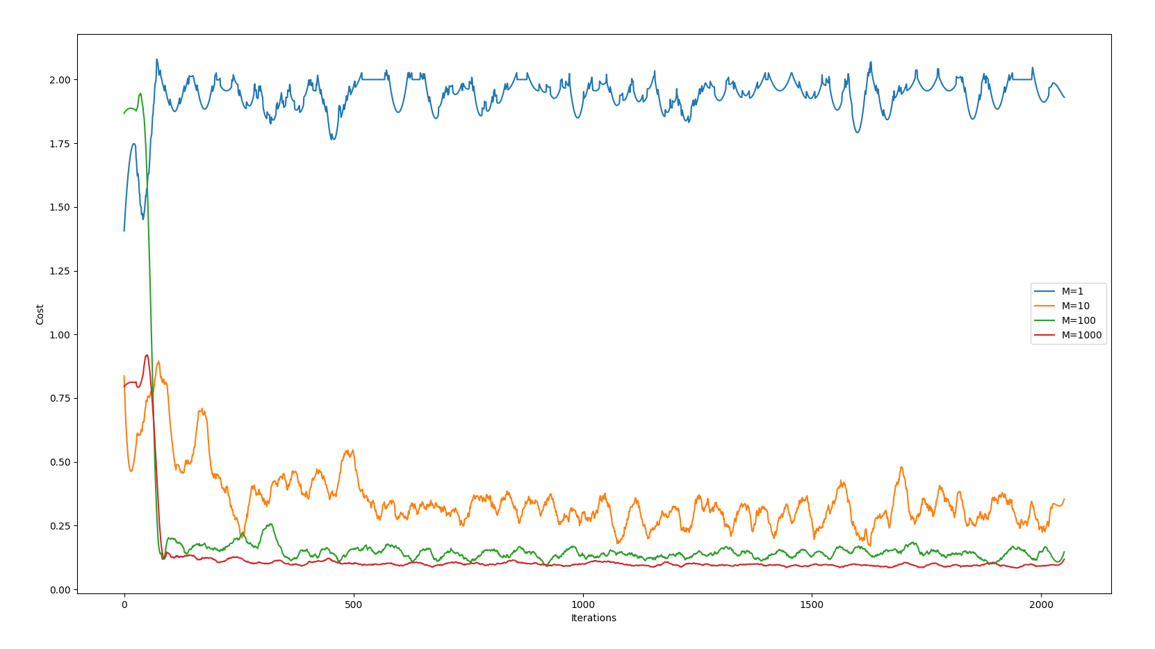
If we plot the costs over time (see diagrams.py) we get the following:

M=1 never even attempts to converge, whereas the other trials reach steady-state after 100 iterations or so, with larger M values demonstrating better results.

Bonus Question

Bonus question:

How to make sure you produce state |01> + |10> and not |01> - |10> ?

If we ignore gate errors, then depending on theta_y, the R_y gate can transform the initial |0> qubit into either |0> + |1> or |0> - |1> (ignoring global phase). Other states are already penalized with the optimization strategy given above, so we only need to distinguish between these two states.

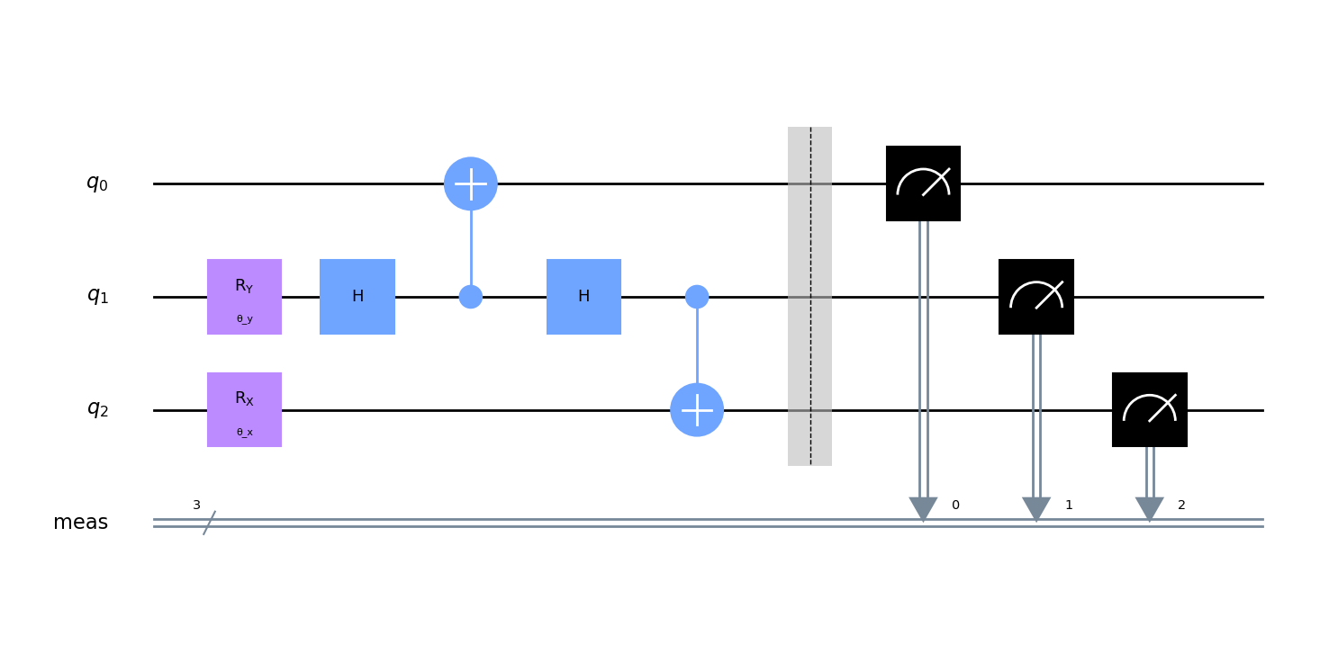
A (maybe somewhat clumsy) method is with the following modified ansatz:

We add a third qubit (initialized as |0>), as well as two Hadamard gates and a CNOT gate. The idea behind this circuit is to act as a "spy" that copies the state of the second qubit without perturbing it. We know the following properties of the Hadamard gate:

    H ( |0> + |1> ) = |0>
    H ( |0> - |1> ) = |1>

as well as the identity H^2 = I. Because of this identity, the second qubit is left unchanged. Meanwhile, the top-most qubit will be |0> if |0> + |1> was produced, and |1> if |0> - |1>. The cost function for the classical optimizer can be adjusted to penalize states wher e the top-most qubit measures anything non-zero.

https://qiskit.org/textbook/ch-applications/vqe-molecules.html#Parameter-Optimization ↩

roytu/qosf_task2