Ryan Burge https://www.ryanburge.net Pkgdown site is available here: https://ryanburge.github.io/socsci/index.html
Instructor of Political Science, Eastern Illinois University, Charleston IL

You can install:
-
the latest development version from GitHub with
install.packages("devtools")
devtools::install_github("ryanburge/socsci")
I love the functionality of tabyl, but it doesn’t take a weight
variable. Here’s the simple version ct()
library(socsci)
cces <- read_csv("https://raw.githubusercontent.com/ryanburge/blocks/master/cces.csv")

cces %>%
  ct(race)
#> # A tibble: 8 x 3
#>    race     n   pct
#>   <dbl> <int> <dbl>
#> 1     1   368 0.736
#> 2     2    54 0.108
#> 3     3    38 0.076
#> 4     4    13 0.026
#> 5     5     7 0.014
#> 6     6     9 0.018
#> 7     7     8 0.016
#> 8     8     3 0.006
Note that you are presented with a count column and a pct column.
Let’s add weights
cces %>%
  ct(race, commonweight_vv)
#> # A tibble: 8 x 3
#>    race       n   pct
#>   <dbl>   <dbl> <dbl>
#> 1     1 348.    0.758
#> 2     2  43.9   0.096
#> 3     3  34.0   0.074
#> 4     4   7.09  0.015
#> 5     5   3.87  0.008
#> 6     6  15.2   0.033
#> 7     7   6.33  0.014
#> 8     8   0.704 0.002
Notice that it’s pipeable. And if you don’t include the weight variable then it won’t be calculated with a weight.
I’ve also added the ability to filter out the NA’s before the calculation is made.
cces %>%
  mutate(race2 = frcode(race == 1 ~ "White",
                        race == 2 ~ "Black",
                        race == 3 ~ "Hispanic",
                        race == 4 ~ "Asian")) %>%
  ct(race2, commonweight_vv)
#> # A tibble: 5 x 3
#>   race2         n   pct
#>   <fct>     <dbl> <dbl>
#> 1 White    348.   0.758
#> 2 Black     43.9  0.096
#> 3 Hispanic  34.0  0.074
#> 4 Asian      7.09 0.015
#> 5 <NA>      26.1  0.057

cces %>%
  mutate(race2 = frcode(race == 1 ~ "White",
                        race == 2 ~ "Black",
                        race == 3 ~ "Hispanic",
                        race == 4 ~ "Asian")) %>%
  ct(race2, show_na = FALSE, commonweight_vv)
#> # A tibble: 4 x 3
#>   race2         n   pct
#>   <fct>     <dbl> <dbl>
#> 1 White    348.   0.804
#> 2 Black     43.9  0.101
#> 3 Hispanic  34.0  0.078
#> 4 Asian      7.09 0.016
This behavior is off by default, however.
Oftentimes in social science we like to see what our 95% confidence
intervals are, but that’s a lot of syntax. It’s easy with the mean_ci
function. I found the basic syntax on a Stack Overflow
post,
from the user
sboysel.
cces %>%
  mean_ci(gender)
#> # A tibble: 1 x 7
#>    mean    sd     n level     se lower upper
#>   <dbl> <dbl> <int> <dbl>  <dbl> <dbl> <dbl>
#> 1  1.54 0.499   500  0.05 0.0223  1.49  1.58
The default is a 95% confidence interval. However that can be changed easily.
cces %>%
  mean_ci(gender, ci = .84)
#> # A tibble: 1 x 7
#>    mean    sd     n level     se lower upper
#>   <dbl> <dbl> <int> <dbl>  <dbl> <dbl> <dbl>
#> 1  1.54 0.499   500  0.16 0.0223  1.50  1.57
This can also take weights.
cces %>%
  mean_ci(gender, ci = .84, wt = commonweight_vv)
#> # A tibble: 1 x 6
#>    mean    sd     n     se lower upper
#>   <dbl> <dbl> <int>  <dbl> <dbl> <dbl>
#> 1 1.50 0.499 500 0.0223 1.47 1.53I wanted a simple function to calculate the mean and the median. It takes just one variable and computes both statistics.
money1 <- read_csv("https://raw.githubusercontent.com/ryanburge/pls2003_sp17/master/sal_work.csv")

money1
#> # A tibble: 1,025 x 3
#>       X1 salary names
#>    <dbl>  <dbl> <chr>
#>  1     1  14736 Darin Casem
#>  2     2  21261 Jaelyn Groesbeck
#>  3     3  16831 Theodis Butler
#>  4     4  34400 Joewid Rettig
#>  5     5  31239 Breianna Gilbert
#>  6     6  51580 Marcus Gray II
#>  7     7  49699 Berenice Garcia
#>  8     8  66805 Elijah Garrett
#>  9     9  49321 Jeremiah Bishop Jr
#> 10    10  67126 Sultana al-Jabbour
#> # ... with 1,015 more rows

money1  %>%
  mean_med(salary)
#> # A tibble: 1 x 2
#>       mean median
#>      <dbl>  <dbl>
#> 1 1247953. 35853Here’s a simple function that generates a pearson correlation of two variables with a p-value.
x <- c(1, 2, 3, 7, 5, 777, 6, 411, 8)
y <- c(11, 23, 1, 4, 6, 22455, 34, 22, 22)
z <- c(34, 3, 21, 4555, 75, 2, 3334, 1122, 22312)

test <- data.frame(x,y,z) %>% as.tibble()

test %>%
  filter(z > 10) %>%
  corr(x,y)
#> # A tibble: 1 x 8
#>   estimate statistic p.value     n conf.low conf.high method                               alternative
#>      <dbl>     <dbl>   <dbl> <int>    <dbl>     <dbl> <chr>                                <chr>
#> 1 0.288 0.673 0.531 5 -0.594 0.856 Pearson's product-moment correlation two.sidedOftentimes I make many little dataframes that I need to bind_rows to put into one large dataframe. As long as those dataframes have the same naming convention that can be done.
dd1 <- data.frame(a = 1, b = 2)
dd2 <- data.frame(a = 3, b = 4)
dd3 <- data.frame(a = 5, b = 6)

bind_df("dd")
#>   a b
#> 1 1 2
#> 2 3 4
#> 3 5 6I recode all the time, but unfortunately when you recode from numeric to
character the factor levels are plotted in alphabetical order. There’s a
way around that now. This uses the case_when function from dplyr but
makes sure that the factors level are the same order of how they are
specified in the function.
I found this terrific function written by Dennis YL, where he had the same problem that I had.
cces <- read_csv("https://raw.githubusercontent.com/ryanburge/cces/master/CCES%20for%20Methods/small_cces.csv")

graph <- cces %>%
  mutate(pid_new = frcode(pid7 == 1 ~ "Strong Democrat",
                          pid7 == 2 ~ "Not Strong Democrat",
                          pid7 == 3 ~ "Lean Democrat",
                          pid7 == 4 ~ "Independent",
                          pid7 == 5 ~ "Lean Republican",
                          pid7 == 6 ~ "Not Strong Republican",
                          pid7 == 7 ~ "Strong Republican",
                          TRUE ~ "REMOVE")) %>%
  ct(pid_new)


graph %>%
  filter(pid_new != "REMOVE") %>%
  ggplot(., aes(x = pid_new, y = pct)) +
  geom_col()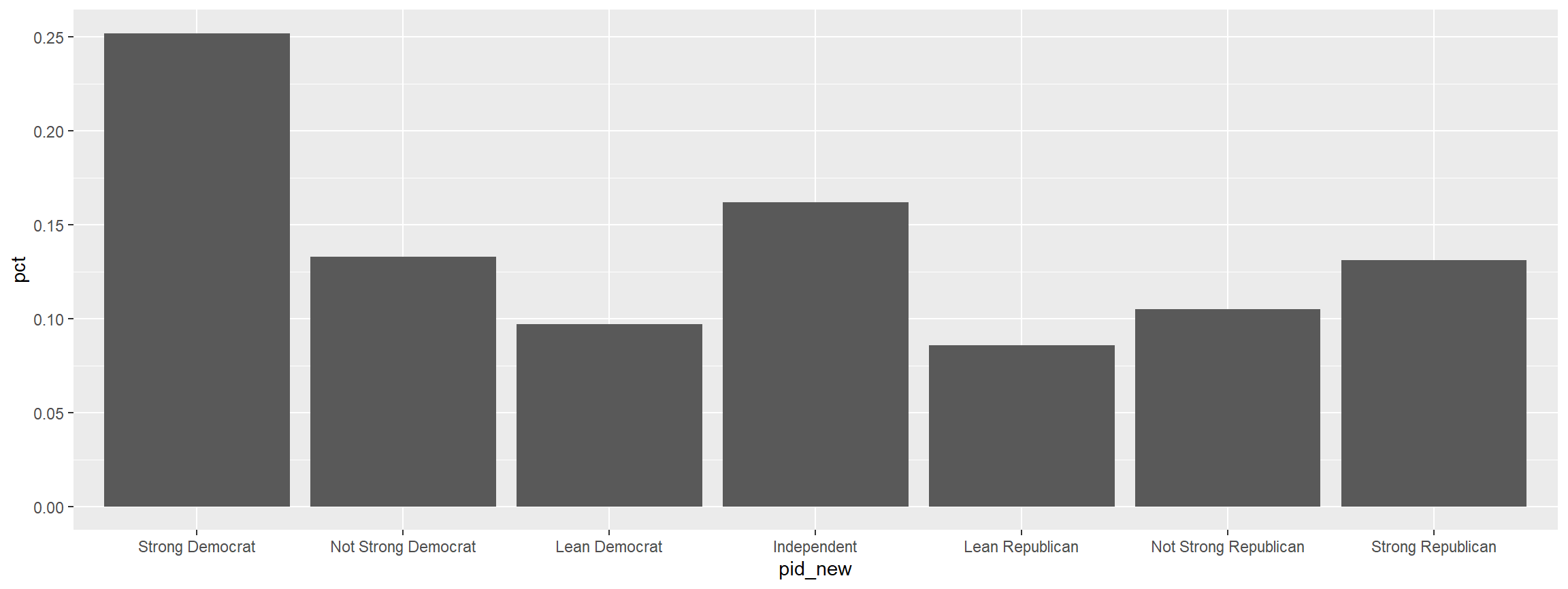
Making a crosstab is one of the building blocks of social science statistics. This function visualizes that crosstab. The first variable is the one that is grouped and the second is the one that is counted
cces %>%
  mutate(pid_new = frcode(pid7 == 1 ~ "Strong Democrat",
                          pid7 == 2 ~ "Not Strong Democrat",
                          pid7 == 3 ~ "Lean Democrat",
                          pid7 == 4 ~ "Independent",
                          pid7 == 5 ~ "Lean Republican",
                          pid7 == 6 ~ "Not Strong Republican",
                          pid7 == 7 ~ "Strong Republican",
                          TRUE ~ "All Others")) %>%
  mutate(gender = frcode(gender ==1 ~ "Male",
                         gender ==2 ~ "Female")) %>%
xheat(gender, pid_new) 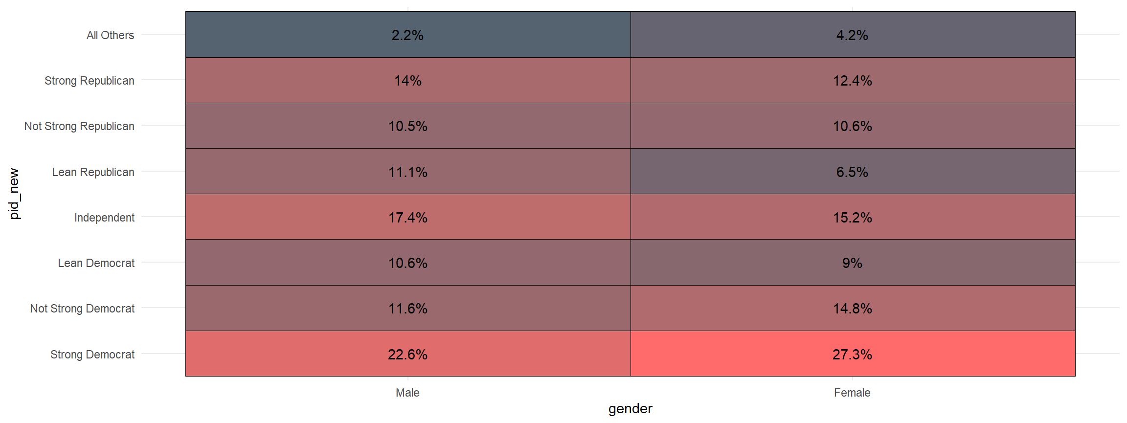
And, you can quickly add the sample size to the graph.
cces %>%
  mutate(pid_new = frcode(pid7 == 1 ~ "Strong Democrat",
                          pid7 == 2 ~ "Not Strong Democrat",
                          pid7 == 3 ~ "Lean Democrat",
                          pid7 == 4 ~ "Independent",
                          pid7 == 5 ~ "Lean Republican",
                          pid7 == 6 ~ "Not Strong Republican",
                          pid7 == 7 ~ "Strong Republican",
                          TRUE ~ "All Others")) %>%
  mutate(gender = frcode(gender ==1 ~ "Male",
                         gender ==2 ~ "Female")) %>%
xheat(gender, pid_new, count = TRUE) 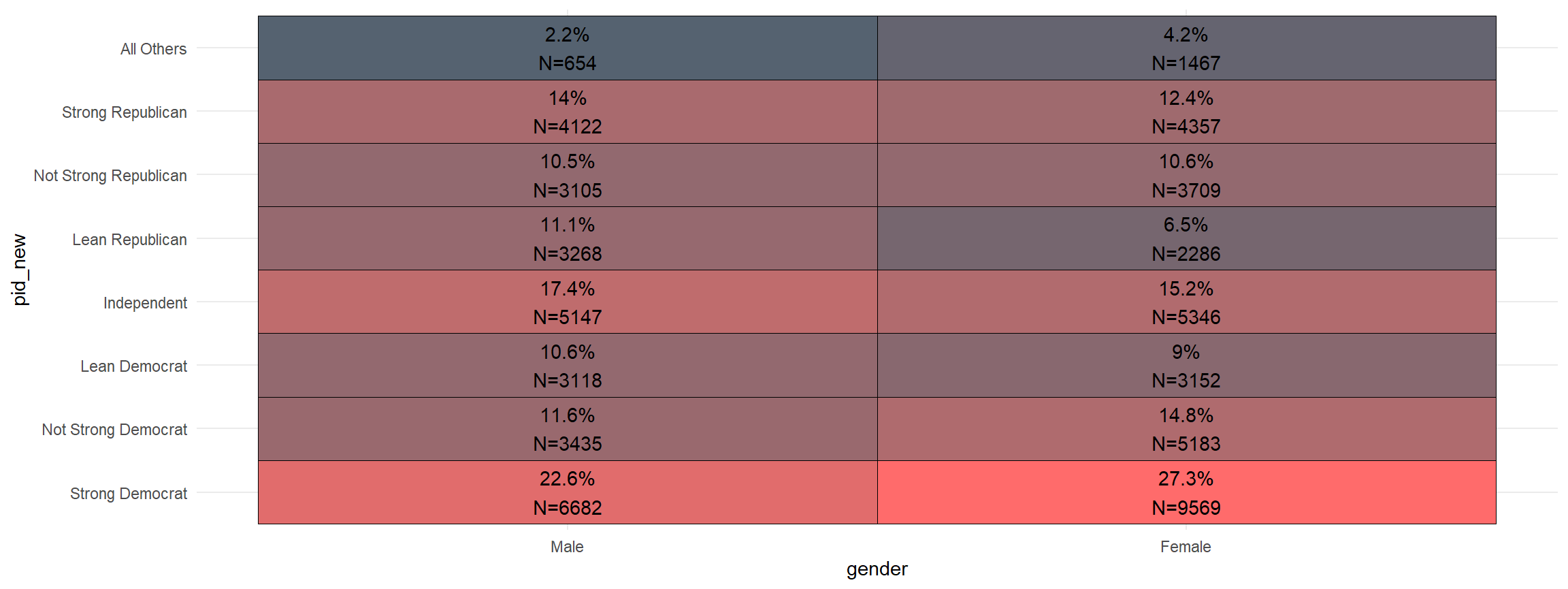
- let me know what you think on twitter @ryanburge