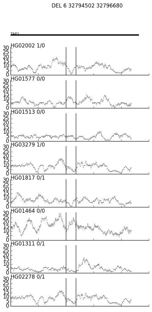
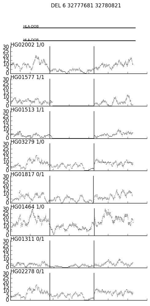
A two-step process that can help visualize the coverage near a variant across multiple BAMs.
Step 1: Create a coverage file for each variant in a VCF. (NOTE: use GQT, bcftools, bedtools etc to filter your full VCF down to a more interesting/managable subset.)
$ bcftools view test/test.vcf.gz | ./sv_depth.py test/test.ped 1000
sv_depth.py creates a covrage file "var_ID.txt" for each SV in the VCF, where ID is the variant ID (3rd column of the variant record). In this case, test/test.vcf.gz has two variants, DEL_pindel_18715 and UW_VH_5456, and so it creates var_DEL_pindel_18715.txt and var_UW_VH_5456.txt. The two parameters to sv_depth.py are the ped file (where the 8th column is a path to the BAM files) and a the distance up and down stream of the the SV that is inclued in the coverage file.
Step 2: Visualize these coverages with spark.py, which takes an exome file, a map from transcrip to gene name, and an ouputfile.
$ cat var_DEL_pindel_18715.txt \
    | ./spark.py \
        -e data/h37_ensemble_exons.bed.gz \
        -n data/h37_ensemble_exons.togenename.txt \
        -o var_DEL_pindel_18715.png
$ cat var_UW_VH_5456.txt \
    | ./spark.py \
        -e data/h37_ensemble_exons.bed.gz \
        -n data/h37_ensemble_exons.togenename.txt \
        -o var_UW_VH_5456.png

