install.packages('tidyquant')
install.packages('fpp2', dependencies=TRUE)
library(tidyquant)
library(fpp2)
library(ggplot2)# Get training data
train_set = tq_get('DMART.NS', from='2014-01-01', to='2019-12-31', get='stock.prices')
test_set = tq_get('DMART.NS', from='2020-05-01', to='2020-05-31', get='stock.prices')head(train_set)head(test_set)train_set %>%
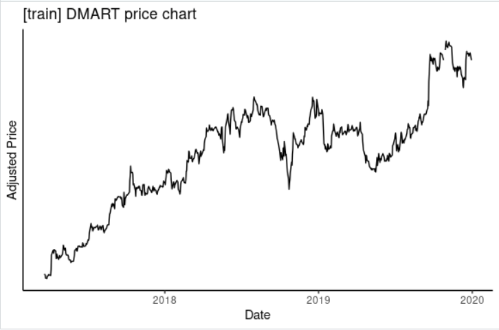
ggplot(aes(x = date, y = adjusted)) +
geom_line() +
theme_classic() +
labs(x = 'Date',
y = "Adjusted Price",
title = "[train] DMART price chart") +
scale_y_continuous(breaks = seq(0,300,10))test_set %>%
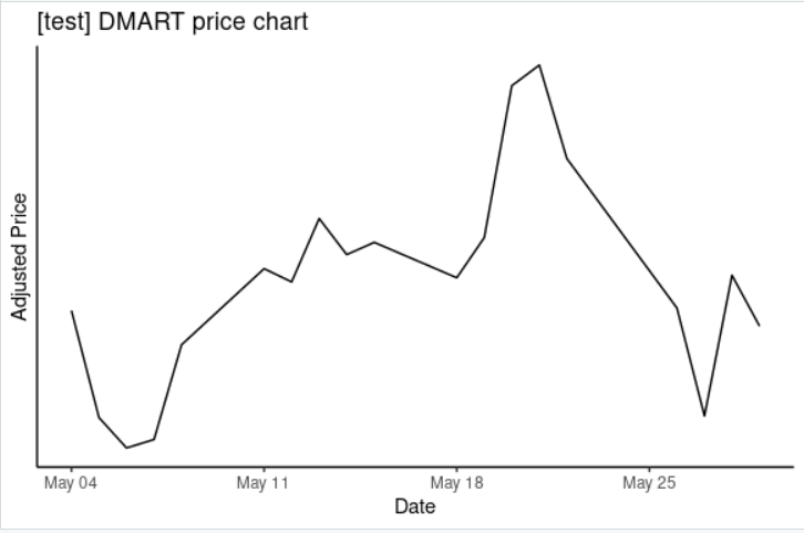
ggplot(aes(x = date, y = adjusted)) +
geom_line() +
theme_classic() +
labs(x = 'Date',
y = "Adjusted Price",
title = "[test] DMART price chart") +
scale_y_continuous(breaks = seq(0,300,10))We are using order 2
train_cleaned = subset(train_set, select = -c(close, high, low, open, symbol, volume))
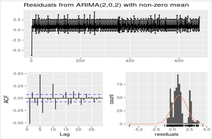
(fit <- data=train_cleaned )autoplot(fit)autoplot(forecast(fit, h=150))Plot of test data
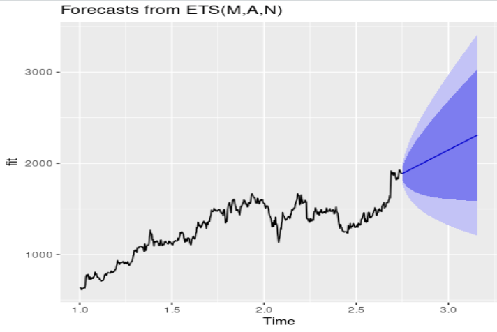
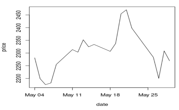
Forecast of fit shows that the price of NSE:DMART potentially lies approximately between 1600 and 3000. Throughout the test period it can be seen that the price lies between 2100 and 2500, which is a subset of 1600-3000.


