This repository contains Python code that implements a restricted Boltzmann machine and performs several tests using the MNIST dataset and Landsat satellite images. The code here was primarily written as an exercise to learn about RBMs and their properties.
The code is capable of running 3 types of model, each of which is trained on training images and applied to test images: * A multinomial regression on the image pixels * An RBM followed by a multinomial regression on the hidden nodes. The RBM is first trained on the image data without using the labels, and then the hidden node values are fed into the regression model (which uses the image labels) * A multi-layer RBM followed by a multinomial regression on the final layer hidden nodes. The idea behind stacking multiple RBMs is that the final layer can form a representation of the data that a simple regression model can more accurately classify. An additional backpropagation step can be used to fine-tune the weights. [MNIST](http://yann.lecun.com/exdb/mnist) is a standard dataset used to benchmark machine learning algorithms and consists of 28x28 pixel images of handwritten digits, 0-9, with corresponding labels. There are 60,000 training images and 10,000 test images and the aim is to correctly identify the digit in each test image. The MNIST data is not included in this repository and is assumed to be in a subdirectory named "common". Results using alternate methods (many of which achieve higher classification accuracy) can be found [here](http://yann.lecun.com/exdb/mnist).Two activation functions were tested, a logistic function and a rectilinear function. An RBM with 150 hidden nodes was trained for 20,000 iterations using batches of 500 images. The learning rate was 0.01 with a weight decay parameter of 0.01. No attempt was made to optimize the batch size, learning rate, or weight decay. However, the contrastive-divergence error on each iteration had plateaued by completion.
Using only multinomial regression an accuracy (defined as number of images correctly identified / total number of images) of 92.42% was achieved. Using multinomial regression on the hidden nodes of the RBM the accuracy was 90.15% with the logistic activation function and 92.83% with the rectilinear function (the statistical significance of the difference in accuracy was not investigated).
Number of hidden nodes
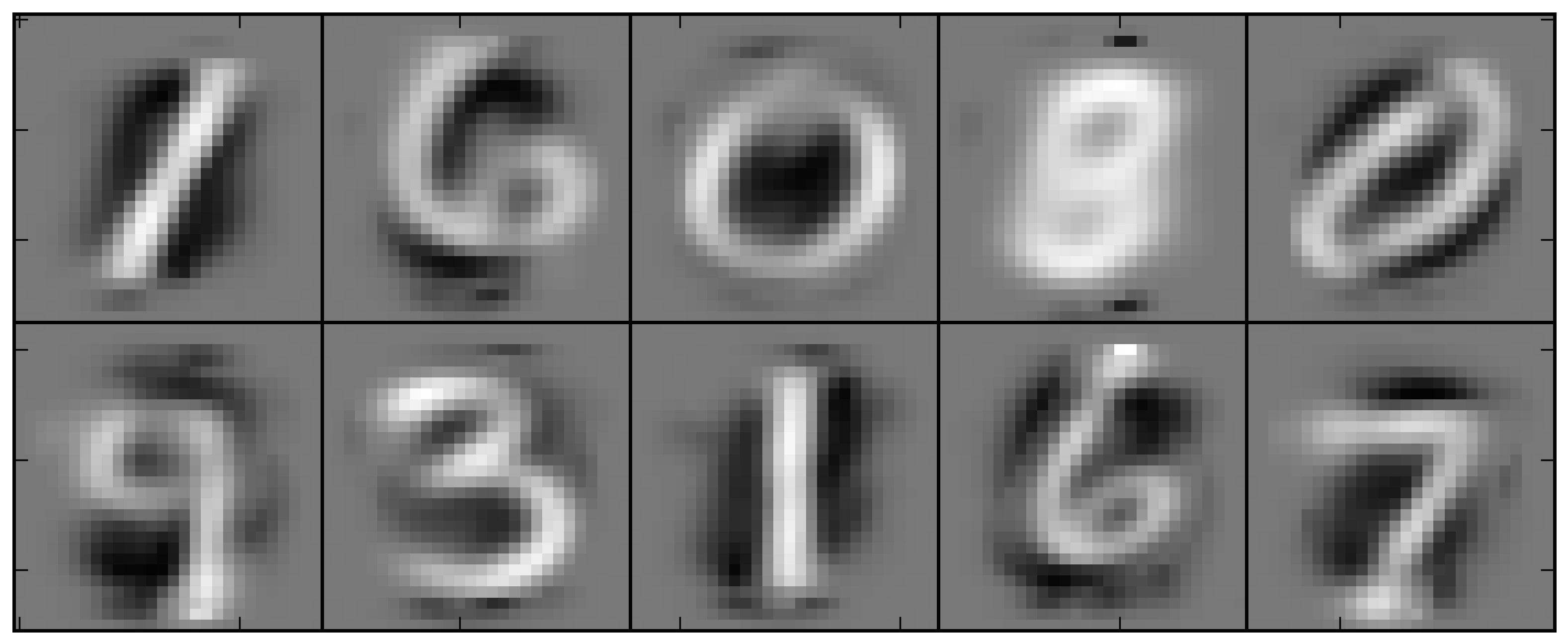
The weights are learned by the RBM without using any of the image labels. Remarkably the values of the hidden nodes give a good representation of the data--even with only 10 hidden nodes the network learns to capture the main features of most of the digits. In this case the weights learned are:
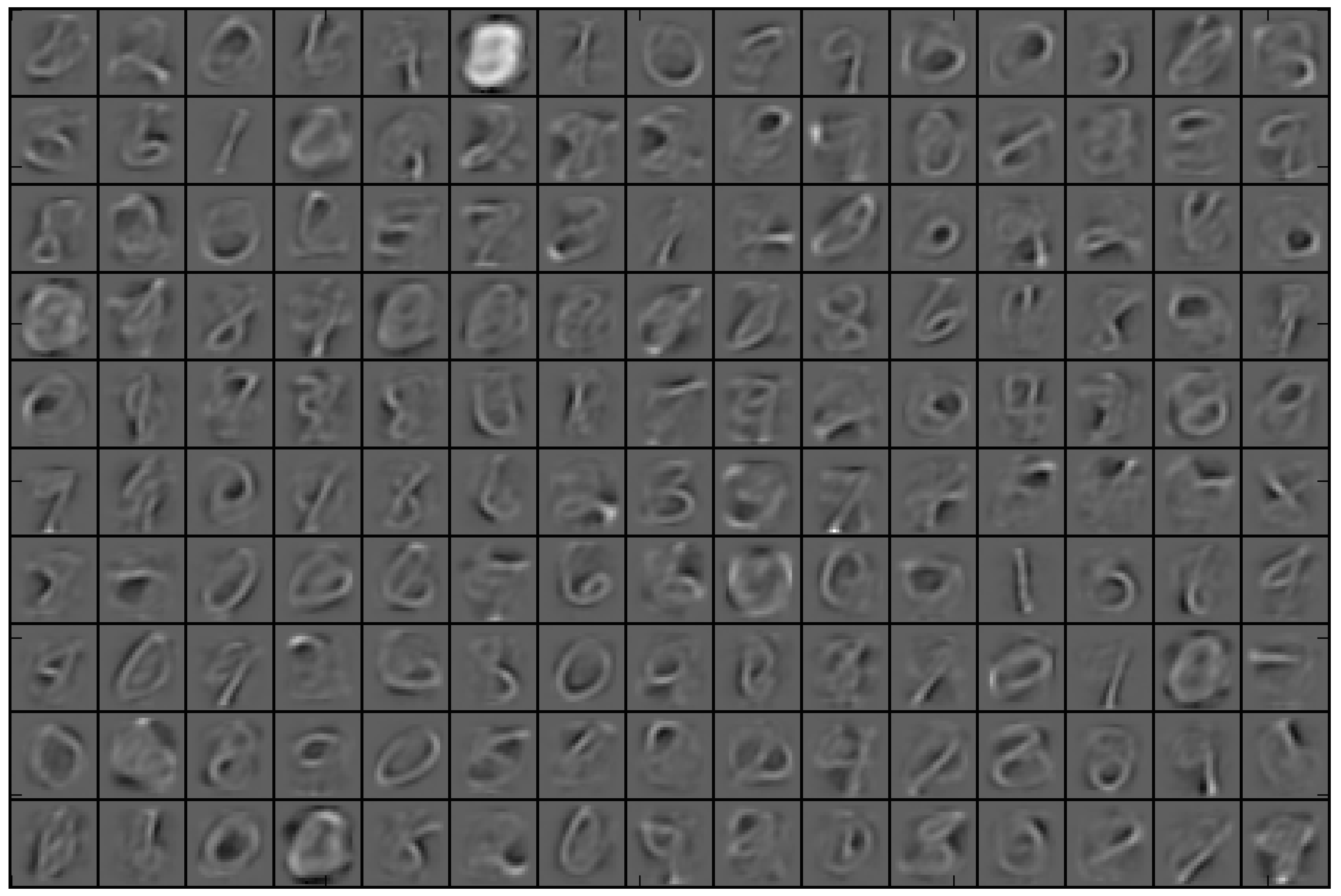
Each 28x28 pixel block in the figure represents the weights connected to 1 hidden node. The fact that the images are "smooth" is further evidence that the contrastive-divergence algorithm has converged. Using 150 hidden nodes:
With the single-layer RBM the accuracy for different network sizes is:
| Number of hidden nodes | Accuracy [%] |
|---|---|
| 784 | 89.58 |
| 350 | 91.94 |
| 200 | 91.70 |
| 150 | 92.83 |
| 50 | 84.38 |
| 10 | 49.17 |
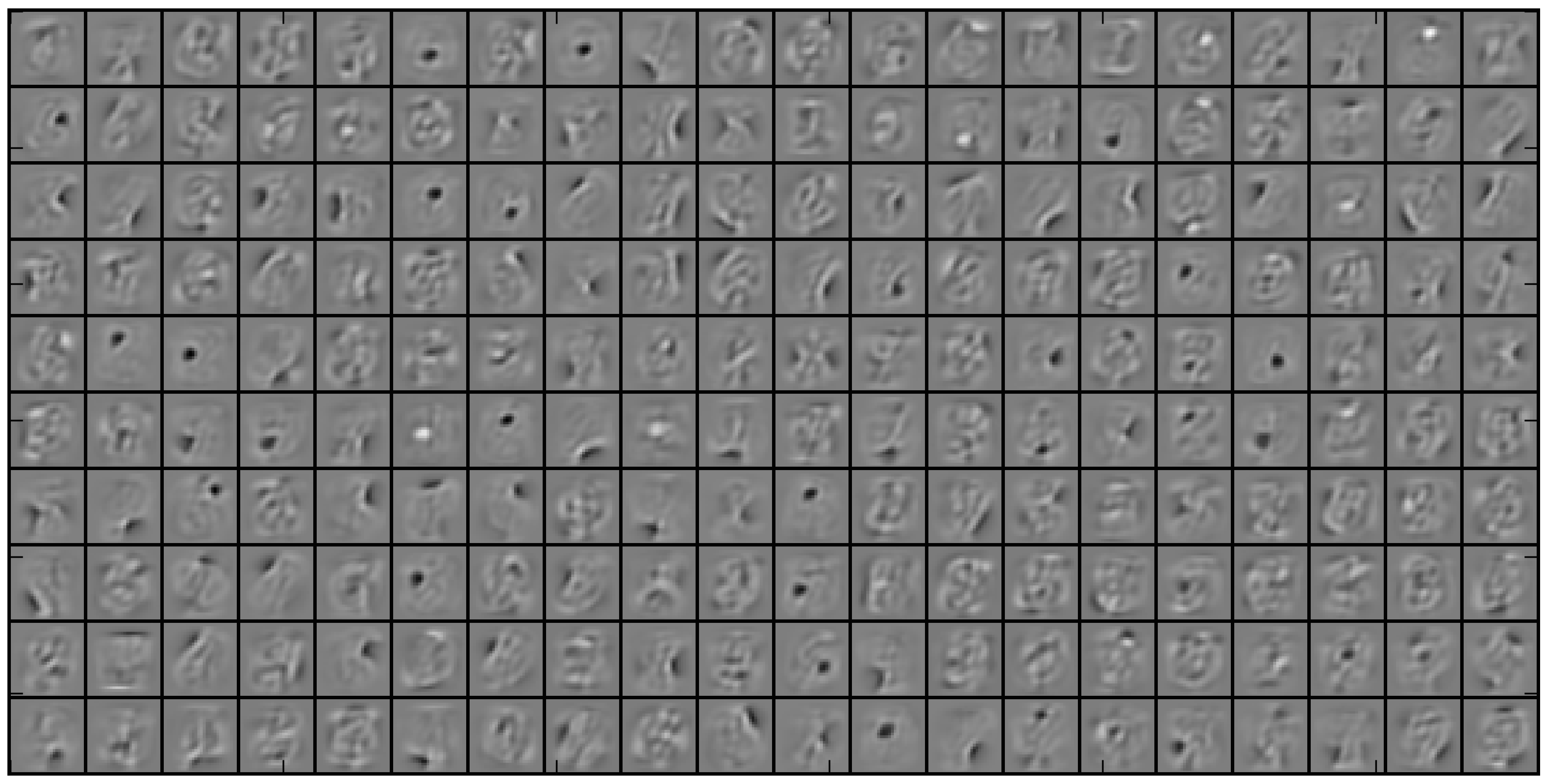
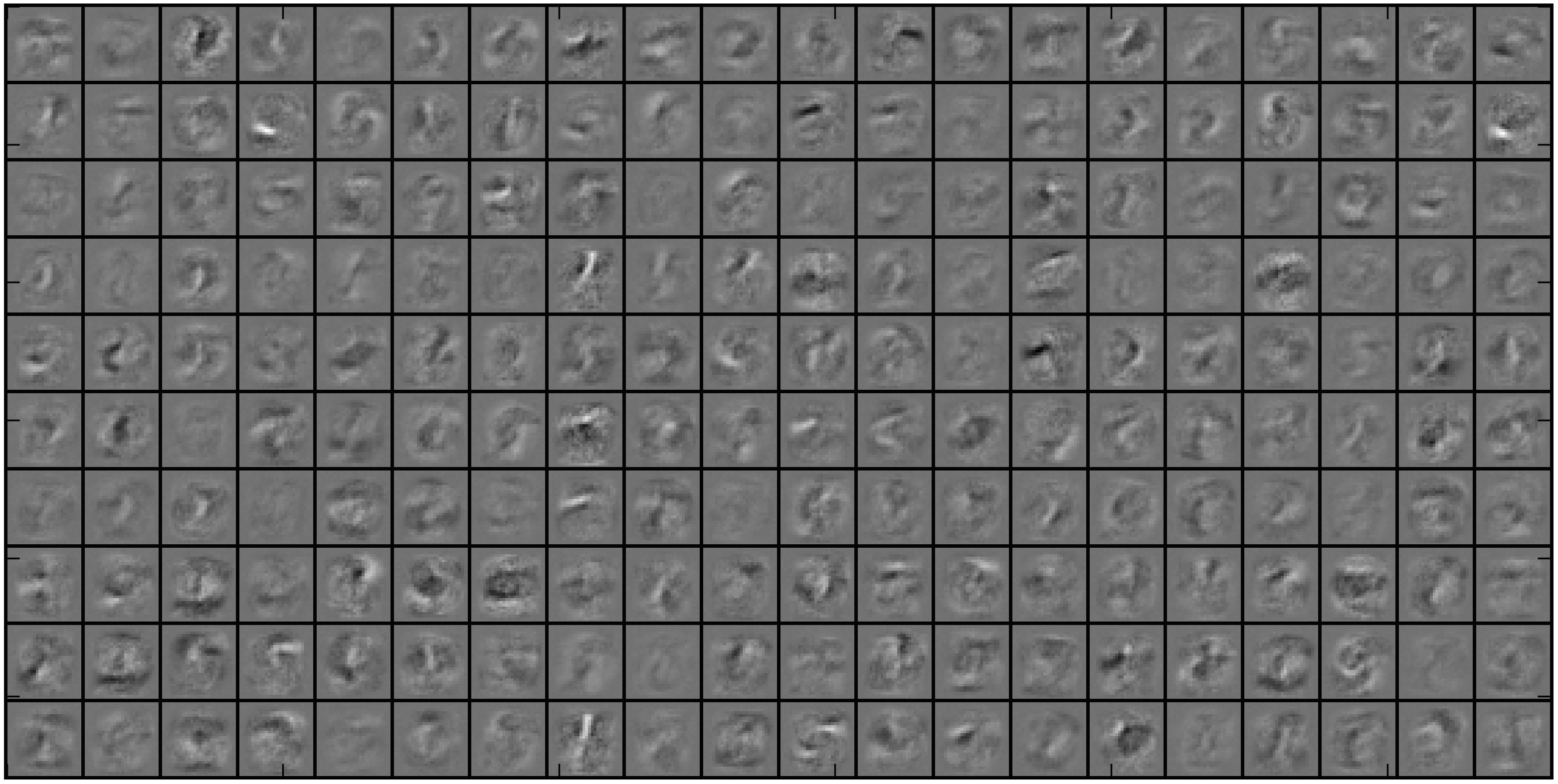
To test the multi-layer RBM a network was set up with 200 hidden nodes in the first layer and 10 in the second layer, a logistic activation function, and a multinomial regression on the output later. The accuracy was 68.45%, lower than using a single RBM with 200 hidden nodes. Using the backpropagation algorithm to update the weights with a batch size of 10 and learning rate of 0.1 resulted in an accuracy of only 69.0% after convergence, suggesting that the weights were stuck in a local minimum configuration. Running the backpropagation algorithm starting from random initial weights resulted in an accuracy of 97.71%. The weights in the first layer have a very different structure in the two cases:
Weights from RBM:
Weights after backpropagation:
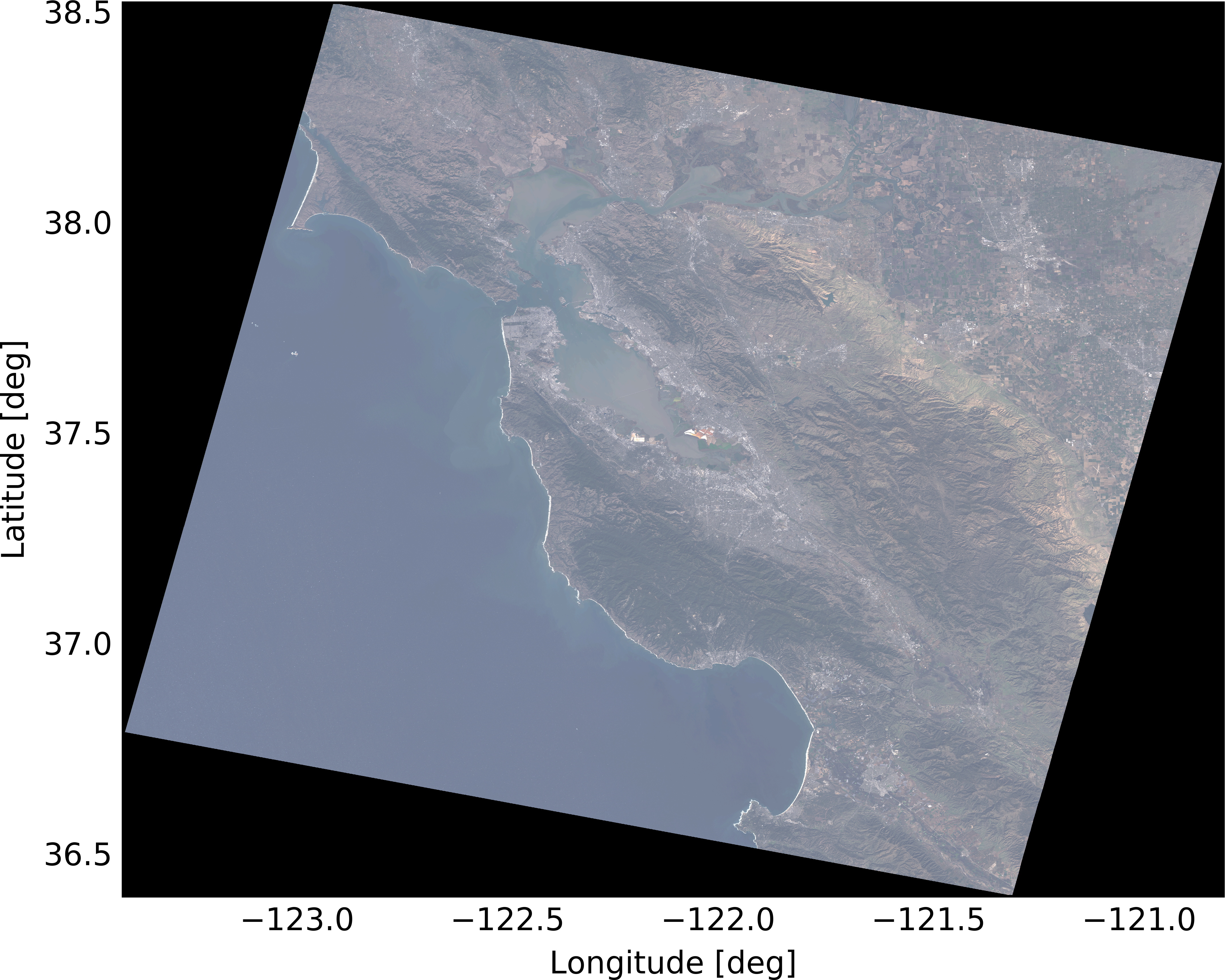
[Landsat](http://landsat.usgs.gov) is a long-running program to obtain satellite-based imagery of the Earth. The most recent satellite, Landsat 8, was launched in February 2013. The following is a Landsat 8 image of the San Francisco bay constructed from the RGB bands and chosen to have less than 4% cloud coverage within the image:The 7811x7671 pixel image was split into 20x20 pixel non-overlapping patches, with each patch normalized to have a peak signal between 0 and 1 (done by selecting the peak signal in any color band so that the color was not distorted). Patches with zero signal were discarded, resulting in 103,000 image patches.
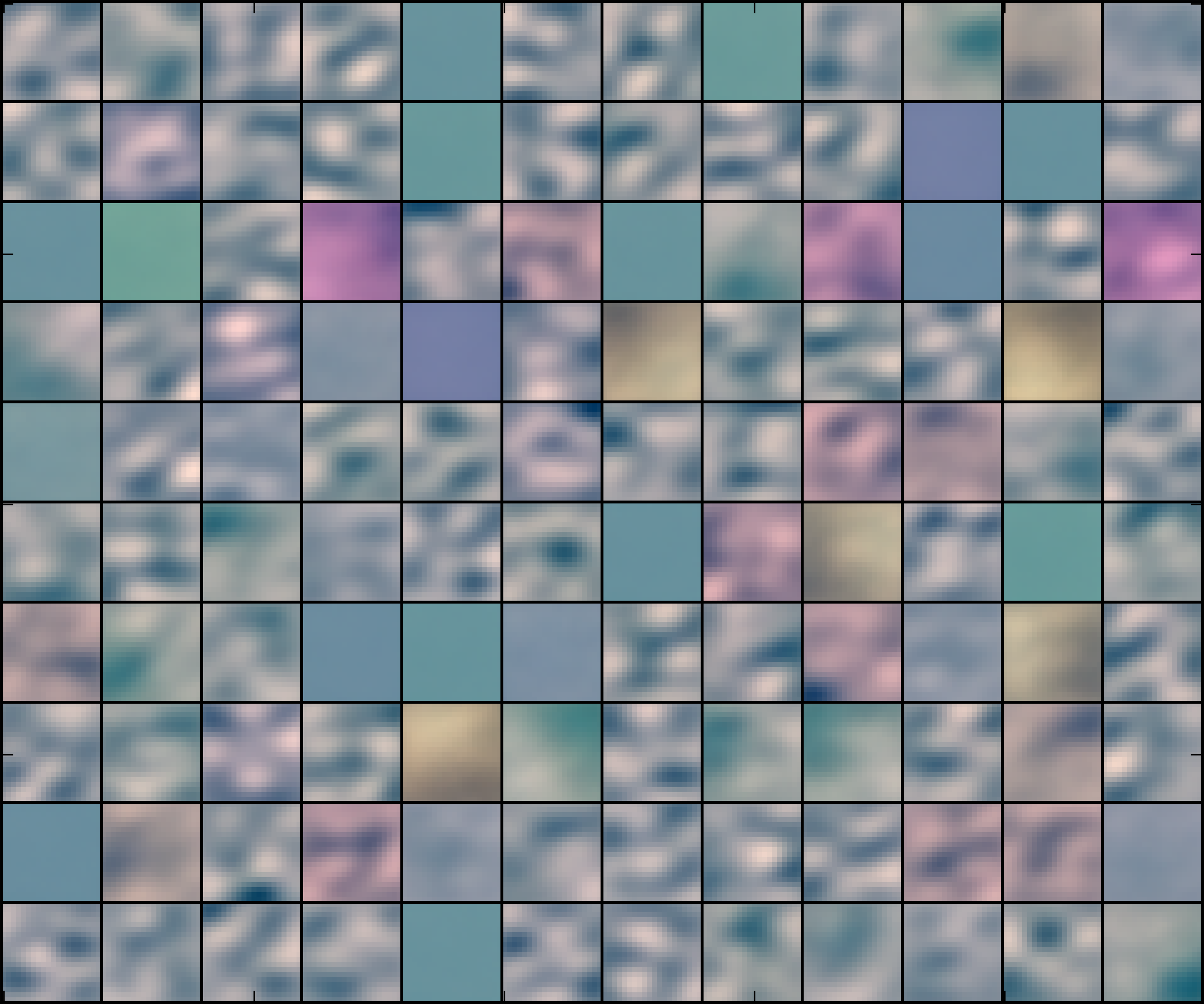
A multi-layer RBM with a 1200-120-120-10 node configuration was trained on the patches. The weights from the first layer show a combination of filters some of which are sensitive to the image structure and some sensitive to the color:
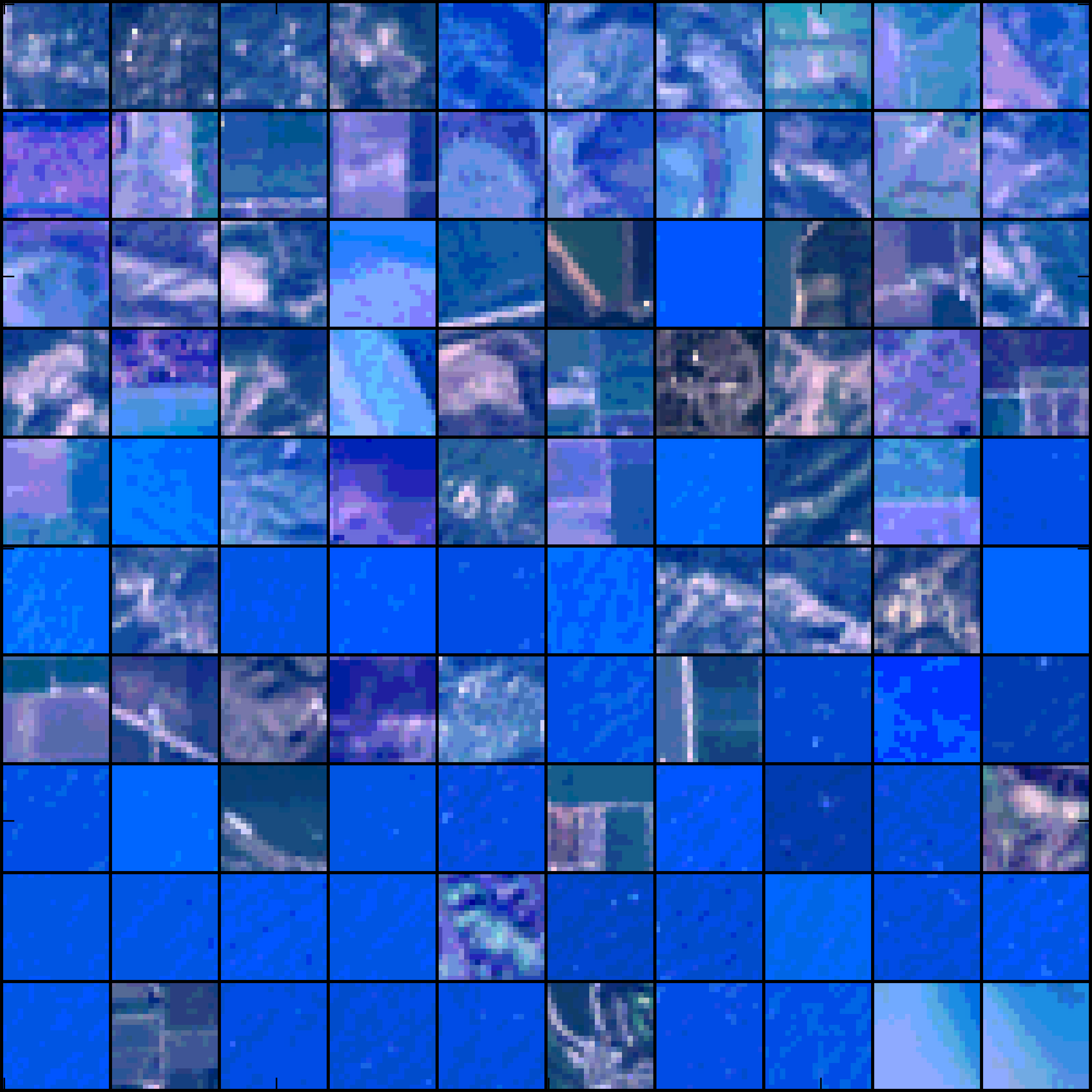
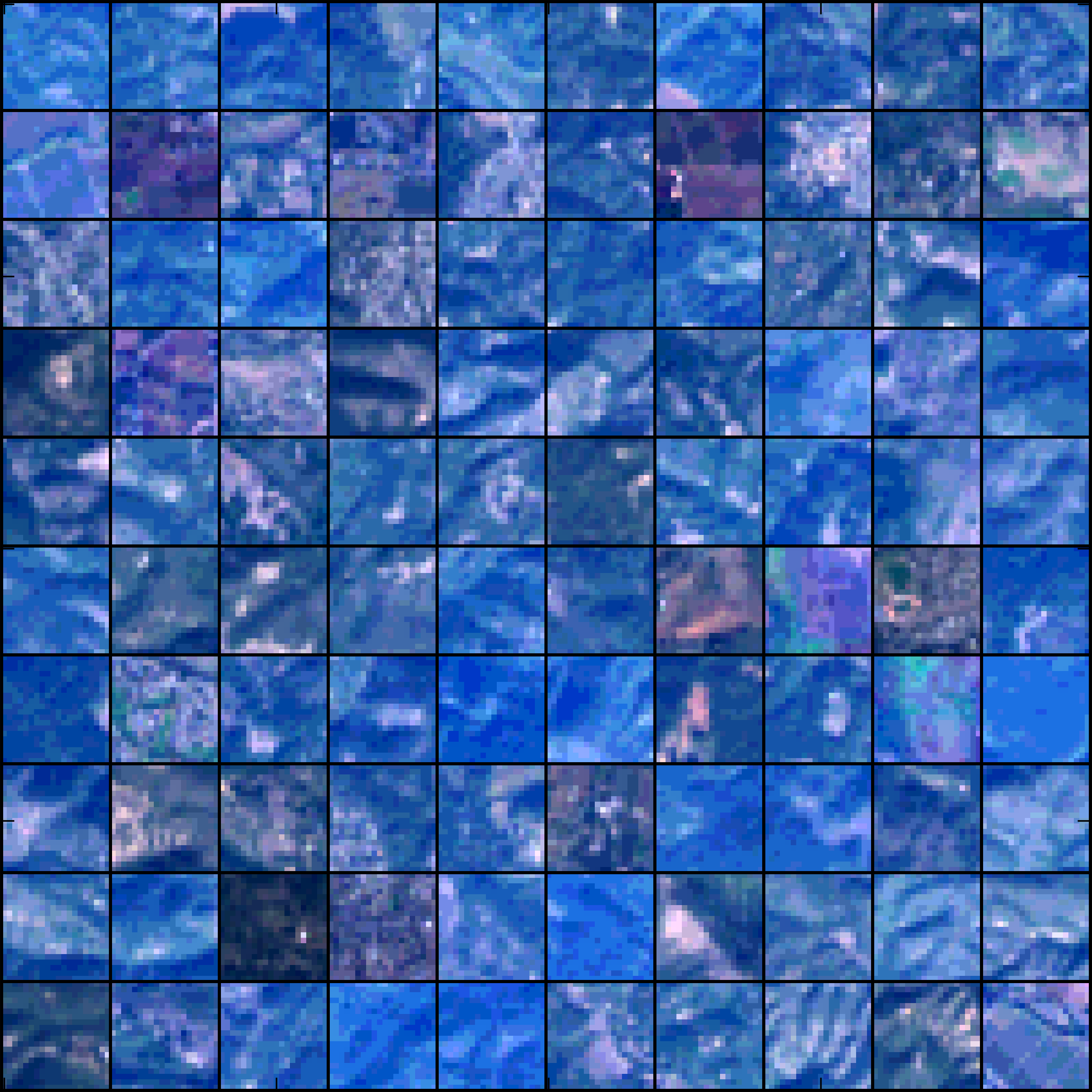
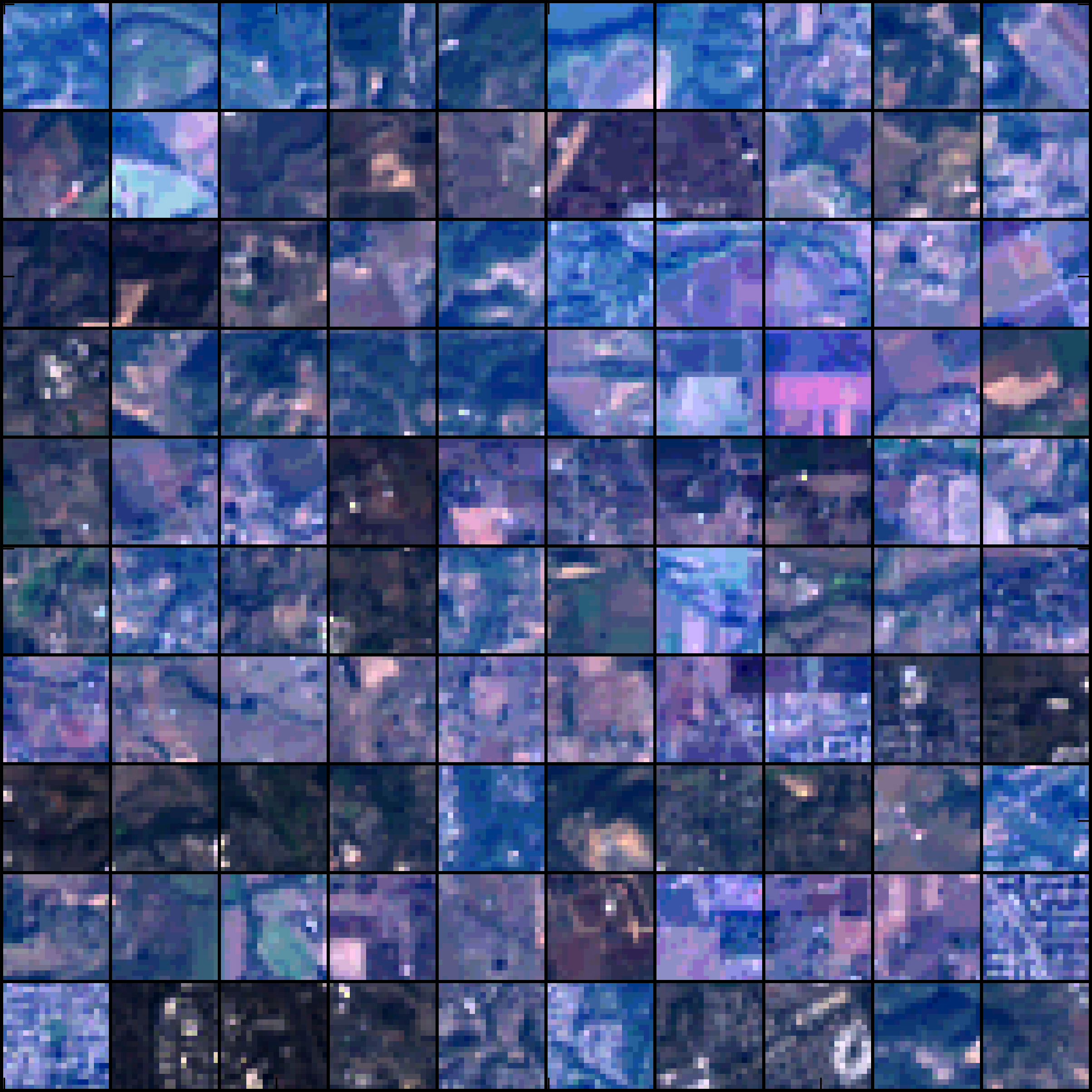
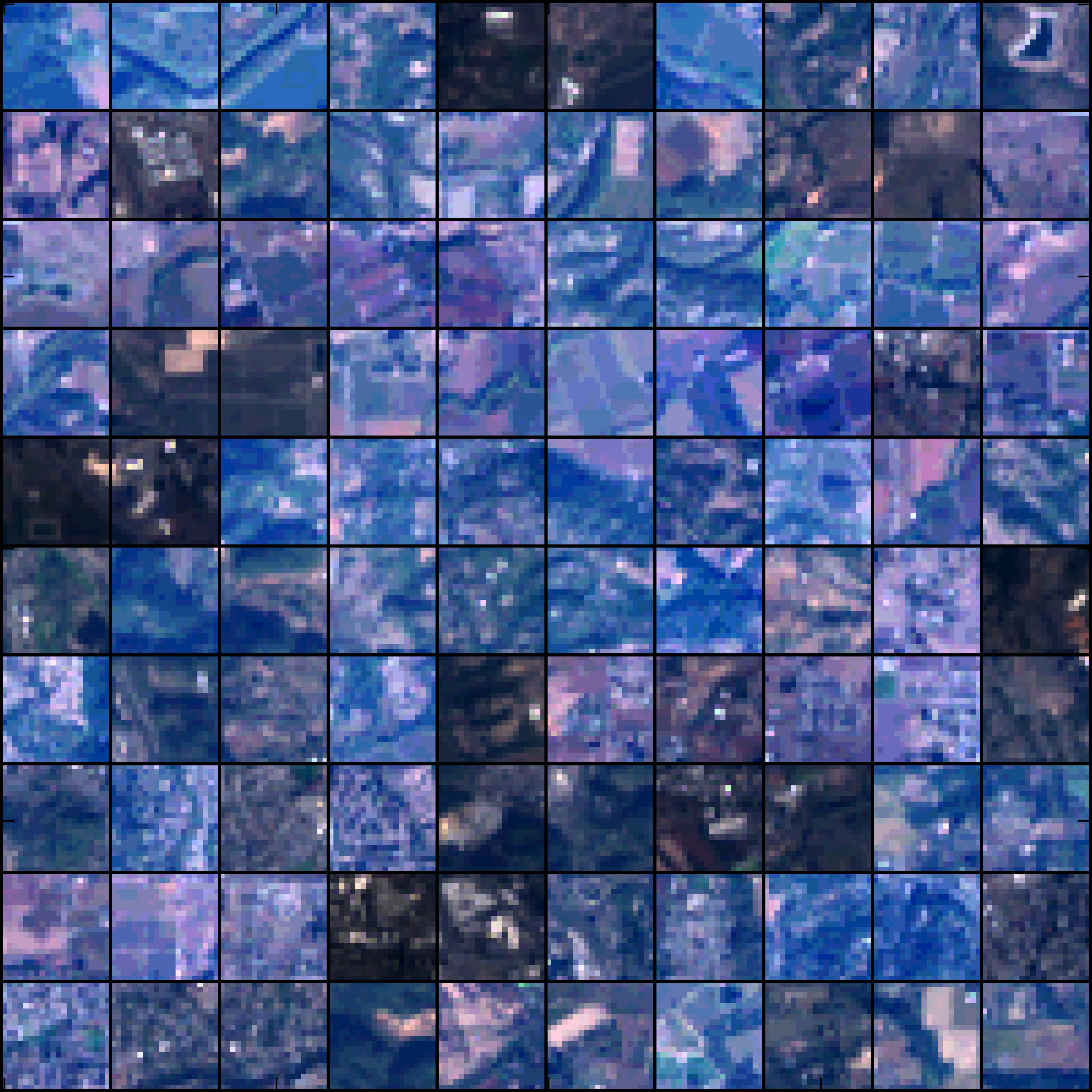
To determine how the RBM classifies the images, the output node with the largest activation signal is selected for each patch. Each image below shows patches that resulted in the same output node having the largest activation:
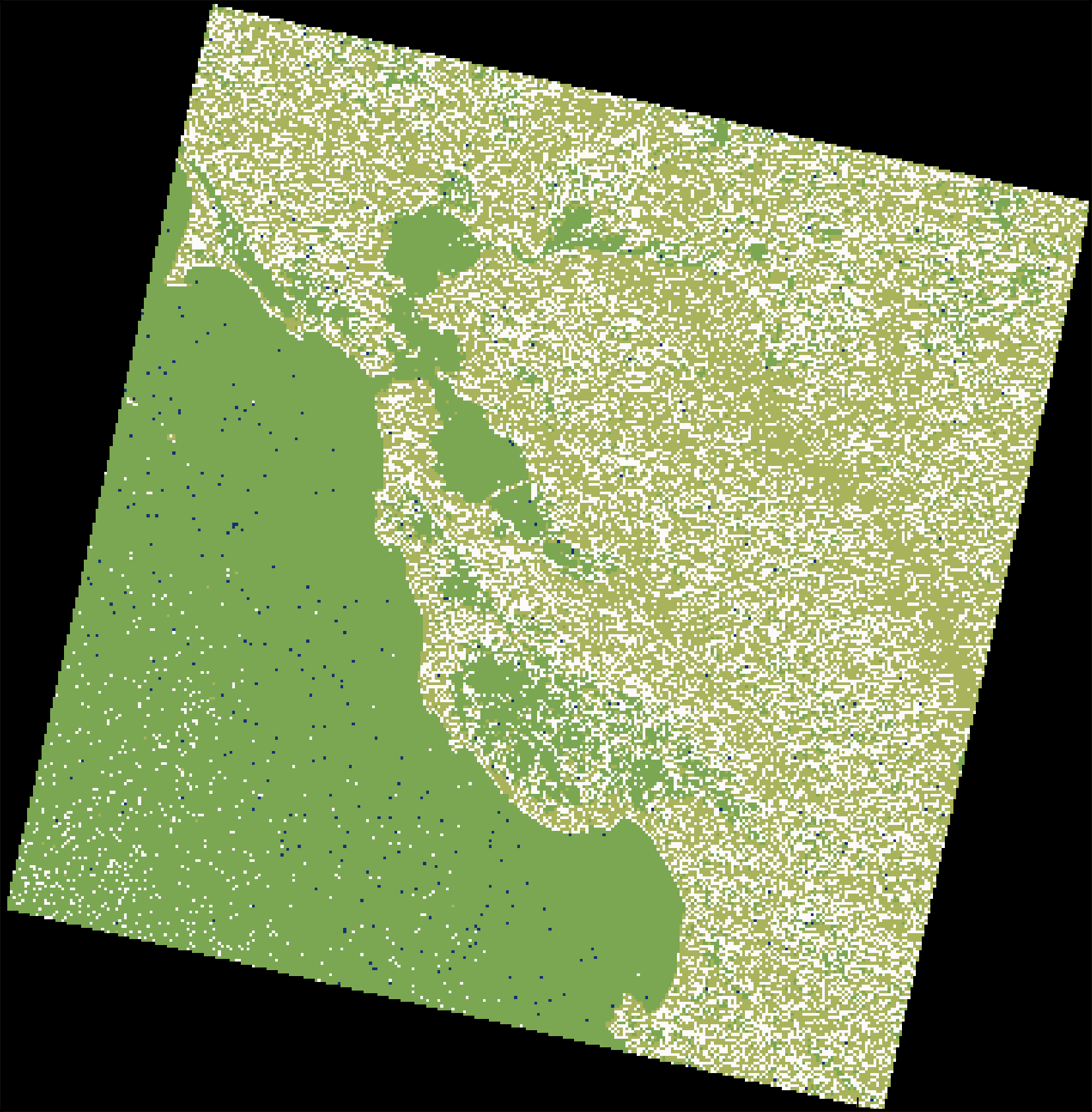
Some of the patches have unnatural looking colors. The patches with strange colors are probably in dark regions or shadowed areas where the color is not accurately determined. Classes 0 and 1 are generally selecting bluer patches (mainly from the ocean) and classes 2 and 3 are selecting purple/brown patches (mainly on land). The geographical distribution of each class is:
