Note: This version of brolgar has been forked from
tprvan/brolgar, and is undergoing
breaking changes to the API.
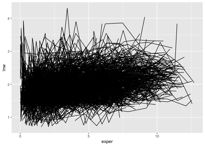
Exploring longitudinal data can be challenging. For example, when there are many individuals it is difficult to look at all of them, as you often get a “plate of spaghetti” plot, with many lines plotted on top of each other.
library(brolgar)
library(ggplot2)
ggplot(wages,
       aes(x = exper,
             y = lnw,
             group = id)) +
  geom_line()
These are hard to interpret.
You might then want to explore those individuals with higher amounts of variation, or those with lower variation. But calculating this for individuals draws you away from your analysis, and instead you are now wrangling with a different problem: summarising key information about each individual and incorporating that back into the data.
This is annoying, and distracts from your analysis, inviting errors.
brolgar (BRowse over Longitudinal data Graphically and Analytically in R) (forked from https://github.com/tprvan/brolgar) provides tools for providing statistical summaries for each individual. These are referred to as a longnostics, a portmanteau of longitudinal and cognostic. These longnostics make it straightforward to extract subjects with certain properties to gain some insight into the data.
Install from GitHub with:
# install.packages("remotes")
remotes::install_github("njtierney/brolgar")Longitudinal data has subjects who are measured on several characteristics repeatedly through time but not always at the same time points or the same number of times.
Let’s extract informative individual patterns by concentrating on different statistics. A story can be woven that may be relevant rather than speaking in generalities.
The wages data set analysed in Singer & Willett (2003) will be used to demonstrate some of the capabilities of this package.
library(brolgar)
library(tibble)
data(wages)
wages
#> # A tibble: 6,402 x 15
#>       id   lnw exper   ged postexp black hispanic   hgc hgc.9 uerate  ue.7
#>    <int> <dbl> <dbl> <int>   <dbl> <int>    <int> <int> <int>  <dbl> <dbl>
#>  1    31  1.49 0.015     1   0.015     0        1     8    -1   3.21 -3.78
#>  2    31  1.43 0.715     1   0.715     0        1     8    -1   3.21 -3.78
#>  3    31  1.47 1.73      1   1.73      0        1     8    -1   3.21 -3.78
#>  4    31  1.75 2.77      1   2.77      0        1     8    -1   3.3  -3.70
#>  5    31  1.93 3.93      1   3.93      0        1     8    -1   2.89 -4.11
#>  6    31  1.71 4.95      1   4.95      0        1     8    -1   2.49 -4.50
#>  7    31  2.09 5.96      1   5.96      0        1     8    -1   2.6  -4.40
#>  8    31  2.13 6.98      1   6.98      0        1     8    -1   4.8  -2.20
#>  9    36  1.98 0.315     1   0.315     0        0     9     0   4.89 -2.10
#> 10    36  1.80 0.983     1   0.983     0        0     9     0   7.4   0.4
#> # … with 6,392 more rows, and 4 more variables: ue.centert1 <dbl>,
#> # ue.mean <dbl>, ue.person.cen <dbl>, ue1 <dbl>The longnostics in brolgar all start with l_, and for all
individuals in the data calculate a statistic for each individual
(specified with an id), for some specified variable:
l_n_obs()Number of observationsl_min()Minimuml_max()Maximuml_mean()Meanl_diff()Lagged difference (by default, the first order difference)l_q1()First quartilel_median()Median valuel_q3()Third quartilel_sd()Standard deviationl_slope()Slope and intercept (given some linear model formula)
For example, we can calculate the number of observations with
l_n_obs():
wages_nobs <- l_n_obs(data = wages, id = id)

wages_nobs
#> # A tibble: 888 x 2
#>       id l_n_obs
#>    <int>   <int>
#>  1    31       8
#>  2    36      10
#>  3    53       8
#>  4   122      10
#>  5   134      12
#>  6   145       9
#>  7   155      11
#>  8   173       6
#>  9   206       3
#> 10   207      11
#> # … with 878 more rows
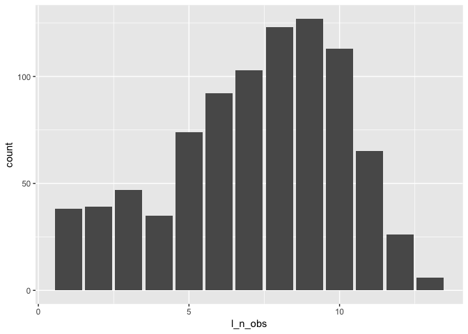
Which could be further summarised to get a sense of the range of the data:
library(dplyr)
#>
#> Attaching package: 'dplyr'
#> The following objects are masked from 'package:stats':
#>
#>     filter, lag
#> The following objects are masked from 'package:base':
#>
#>     intersect, setdiff, setequal, union
library(ggplot2)
ggplot(wages_nobs,
       aes(x = l_n_obs)) +
geom_bar()summary(wages_nobs$l_n_obs)
#> Min. 1st Qu. Median Mean 3rd Qu. Max.
#> 1.000 5.000 8.000 7.209 9.000 13.000We might be interested in showing the experience and lnw (?), and so look at a plot like the following:
ggplot(wages,
       aes(x = exper,
             y = lnw,
             group = id)) +
  geom_line()
This is a plate of spaghetti! It is hard to understand!
We can use brolgar to get the number of observations and slope
information for each individual to identify those that are decreasing
over time.
sl <- l_slope(wages, id, lnw~exper)
ns <- l_n_obs(wages, id)

sl
#> # A tibble: 888 x 3
#>       id l_intercept l_slope_exper
#>    <int>       <dbl>         <dbl>
#>  1    31        1.41        0.101
#>  2    36        2.04        0.0588
#>  3    53        2.29       -0.358
#>  4   122        1.93        0.0374
#>  5   134        2.03        0.0831
#>  6   145        1.59        0.0469
#>  7   155        1.66        0.0867
#>  8   173        1.61        0.100
#>  9   206        1.73        0.180
#> 10   207        1.62        0.0884
#> # … with 878 more rows
ns
#> # A tibble: 888 x 2
#>       id l_n_obs
#>    <int>   <int>
#>  1    31       8
#>  2    36      10
#>  3    53       8
#>  4   122      10
#>  5   134      12
#>  6   145       9
#>  7   155      11
#>  8   173       6
#>  9   206       3
#> 10   207      11
#> # … with 878 more rows
We can then join these summaries back to the data:
wages_lg <- wages %>%
  left_join(sl, by = "id") %>%
  left_join(ns, by = "id")

wages_lg
#> # A tibble: 6,402 x 18
#>       id   lnw exper   ged postexp black hispanic   hgc hgc.9 uerate  ue.7
#>    <int> <dbl> <dbl> <int>   <dbl> <int>    <int> <int> <int>  <dbl> <dbl>
#>  1    31  1.49 0.015     1   0.015     0        1     8    -1   3.21 -3.78
#>  2    31  1.43 0.715     1   0.715     0        1     8    -1   3.21 -3.78
#>  3    31  1.47 1.73      1   1.73      0        1     8    -1   3.21 -3.78
#>  4    31  1.75 2.77      1   2.77      0        1     8    -1   3.3  -3.70
#>  5    31  1.93 3.93      1   3.93      0        1     8    -1   2.89 -4.11
#>  6    31  1.71 4.95      1   4.95      0        1     8    -1   2.49 -4.50
#>  7    31  2.09 5.96      1   5.96      0        1     8    -1   2.6  -4.40
#>  8    31  2.13 6.98      1   6.98      0        1     8    -1   4.8  -2.20
#>  9    36  1.98 0.315     1   0.315     0        0     9     0   4.89 -2.10
#> 10    36  1.80 0.983     1   0.983     0        0     9     0   7.4   0.4
#> # … with 6,392 more rows, and 7 more variables: ue.centert1 <dbl>,
#> #   ue.mean <dbl>, ue.person.cen <dbl>, ue1 <dbl>, l_intercept <dbl>,
#> #   l_slope_exper <dbl>, l_n_obs <int>
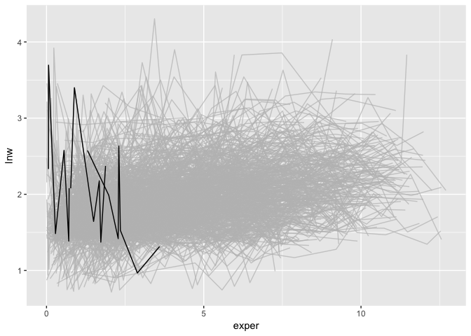
We can then highlight those individuals with more than 5 observations,
and highlight those with a negative slope using gghighlight:
library(gghighlight)

wages_lg %>%
  filter(l_n_obs > 5) %>%
  ggplot(aes(x = exper,
             y = lnw,
             group = id)) +
  geom_line() +
  gghighlight(l_slope_exper < (-0.5),
use_direct_label = FALSE)You can filter by the number of observations using filter_n_obs()
wages %>%
  filter_n_obs(id = id,
               l_n_obs > 3)
#> # A tibble: 6,145 x 16
#>       id l_n_obs   lnw exper   ged postexp black hispanic   hgc hgc.9
#>    <int>   <int> <dbl> <dbl> <int>   <dbl> <int>    <int> <int> <int>
#>  1    31       8  1.49 0.015     1   0.015     0        1     8    -1
#>  2    31       8  1.43 0.715     1   0.715     0        1     8    -1
#>  3    31       8  1.47 1.73      1   1.73      0        1     8    -1
#>  4    31       8  1.75 2.77      1   2.77      0        1     8    -1
#>  5    31       8  1.93 3.93      1   3.93      0        1     8    -1
#>  6    31       8  1.71 4.95      1   4.95      0        1     8    -1
#>  7    31       8  2.09 5.96      1   5.96      0        1     8    -1
#>  8    31       8  2.13 6.98      1   6.98      0        1     8    -1
#>  9    36      10  1.98 0.315     1   0.315     0        0     9     0
#> 10    36      10  1.80 0.983     1   0.983     0        0     9     0
#> # … with 6,135 more rows, and 6 more variables: uerate <dbl>, ue.7 <dbl>,
#> #   ue.centert1 <dbl>, ue.mean <dbl>, ue.person.cen <dbl>, ue1 <dbl>

wages %>%
  filter_n_obs(id = id,
               l_n_obs == 1)
#> # A tibble: 38 x 16
#>       id l_n_obs   lnw exper   ged postexp black hispanic   hgc hgc.9
#>    <int>   <int> <dbl> <dbl> <int>   <dbl> <int>    <int> <int> <int>
#>  1   266       1  1.81 0.322     1   0.182     0        0     9     0
#>  2   304       1  1.84 0.580     0   0         0        1     8    -1
#>  3   911       1  2.51 1.67      1   1.67      1        0    11     2
#>  4  1032       1  1.65 0.808     0   0         1        0     8    -1
#>  5  1219       1  1.57 1.5       0   0         1        0     9     0
#>  6  1282       1  2.22 0.292     1   0.292     0        0    11     2
#>  7  1542       1  1.81 0.173     0   0         0        0    10     1
#>  8  1679       1  1.94 0.365     1   0         0        0    10     1
#>  9  2065       1  2.60 1.5       0   0         0        0    11     2
#> 10  2261       1  2.25 0.005     0   0         0        0     6    -3
#> # … with 28 more rows, and 6 more variables: uerate <dbl>, ue.7 <dbl>,
#> #   ue.centert1 <dbl>, ue.mean <dbl>, ue.person.cen <dbl>, ue1 <dbl>

wages %>%
  filter_n_obs(id = id,
               l_n_obs >= 13)
#> # A tibble: 78 x 16
#>       id l_n_obs   lnw exper   ged postexp black hispanic   hgc hgc.9
#>    <int>   <int> <dbl> <dbl> <int>   <dbl> <int>    <int> <int> <int>
#>  1  1204      13  1.81 0.455     0       0     0        0     8    -1
#>  2  1204      13  1.99 1.28      0       0     0        0     8    -1
#>  3  1204      13  2.08 2.24      0       0     0        0     8    -1
#>  4  1204      13  2.30 3.22      0       0     0        0     8    -1
#>  5  1204      13  2.20 4.20      0       0     0        0     8    -1
#>  6  1204      13  2.33 5.18      0       0     0        0     8    -1
#>  7  1204      13  2.44 6.20      0       0     0        0     8    -1
#>  8  1204      13  2.58 7.28      0       0     0        0     8    -1
#>  9  1204      13  2.22 8.43      0       0     0        0     8    -1
#> 10  1204      13  2.80 9.64      0       0     0        0     8    -1
#> # … with 68 more rows, and 6 more variables: uerate <dbl>, ue.7 <dbl>,
#> # ue.centert1 <dbl>, ue.mean <dbl>, ue.person.cen <dbl>, ue1 <dbl>You can calculate all longnostics using longnostic_all():
longnostic_all(data = wages,
               id = id,
               var = lnw,
               formula = lnw~exper)
#> # A tibble: 888 x 12
#>       id l_diff_1 l_max l_mean l_median l_min l_n_obs  l_q1  l_q3  l_sd
#>    <int>    <dbl> <dbl>  <dbl>    <dbl> <dbl>   <int> <dbl> <dbl> <dbl>
#>  1    31    0.377  2.13   1.75     1.73 1.43        8  1.49  1.97 0.277
#>  2    36    1.11   2.93   2.33     2.32 1.80       10  2.05  2.54 0.387
#>  3    53    1.70   3.24   1.89     1.71 1.54        8  1.59  1.88 0.562
#>  4   122    1.68   2.92   2.17     2.19 0.763      10  2.12  2.42 0.574
#>  5   134    0.368  2.93   2.48     2.36 2.00       12  2.29  2.77 0.321
#>  6   145    0.289  2.04   1.76     1.77 1.48        9  1.60  1.88 0.185
#>  7   155    0.627  2.64   2.17     2.22 1.54       11  1.93  2.40 0.362
#>  8   173    0.319  2.34   1.93     2.00 1.56        6  1.76  2.02 0.274
#>  9   206    0.269  2.48   2.27     2.30 2.03        3  2.16  2.39 0.228
#> 10   207    0.399  2.66   2.11     2.15 1.58       11  1.90  2.24 0.327
#> # … with 878 more rows, and 2 more variables: l_intercept <dbl>,
#> # l_slope_exper <dbl>This version of brolgar has been forked from tprvan/brolgar, and is undergoing breaking changes to the API.


