This UC Berkeley Master of Information in Data Science W207 final project was developed by Spyros Garyfallos, Brent Biseda, and Mumin Khan.
- Project Overview
- Technologies
- Background
- Data Preparation
- Results
- Conclusion
- Installation
- References
This project aims to classify the NIH chest x-ray dataset through the use of a deep neural net architecture. We optimize our model through incremental steps. We first tune hyperparameters, then experiment with different architectures, and ultimately create our final model. The motivation behind this project is to replicate or improve upon the results as laid out in the following paper: ChestX-ray8: Hospital-scale Chest X-ray Database and Benchmarks on Weakly-Supervised Classification and Localization of Common Thorax Diseases.
The workflow for this project is based on the that as laid out by Chahhou Mohammed, winner of the Kaggle $1 Million prize for price prediction on the Zillow dataset. He systematically builds a simple model and gradually adds more complexity while performing grid-search over the hyperparameters. Here we will perform this same task on the Kaggle dataset for NIH Chest X-ray images. https://github.com/MIDS-scaling-up/v2/blob/master/week07/labs/README.md
This dataset was gathered by the NIH and contains over 100,000 anonymized chest x-ray images from more than 30,000 patients. The data represents NLP analysis of radiology reports and may include areas of lower confidence in diagnoses. As a simplifying assumption, wee assume that based on the size of the dataset, that the dataset is accurate in diagnoses.
One of the difficulties of this problem involves the lack of a "diagnosis confidence" attribute in the data. In addition to a chest X-ray, diagnosis involves patient presentation and history. Further, some physician's diagnoses will not be agreed upon by others. Therefore, it is likely that some of the images are mislabeled.
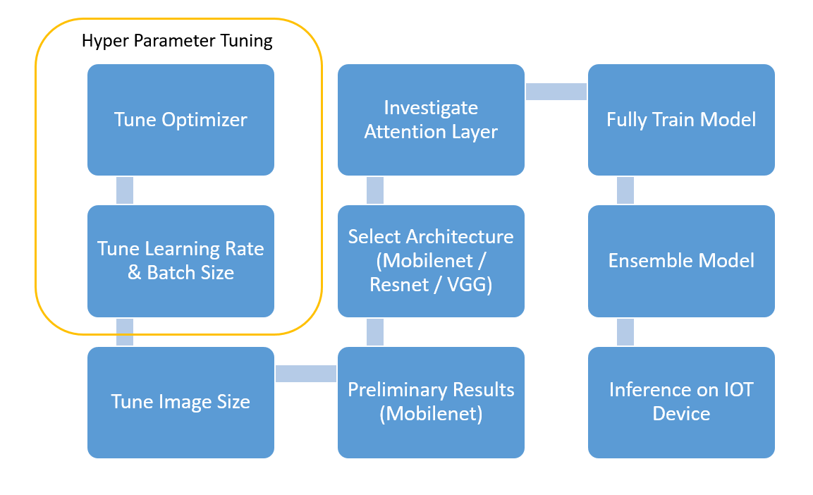
The figure below shows the general roadmap to create our final model.
Convolutional Neural Networks (CNN's) are special types of neural networks that are most often applied to image processing problems. What makes them unique from traditional neural networks is the convolutional layer, a layer in which neurons are connected to pixels only in their receptive fields rather than every single pixel. The result is the ability to extract features while significantly reducing dimensionality. CNN's got their start when two neurophysiologists, David Hubel and Torsten Wiesel, published pioneering research on the response of a cat's visual cortical neurons to stimuli. Soon after, researchers used some of the findings as inspiration for implementing a convolution layer to neural networks. In the 1990's Yann LeCun, Leon Bottou, Yosuha Bengio and Patrick Haffner introduced a groundbreaking algorithm called LeNet-5 for classifying handwritten digits.
LeNet-5 proved to be exceedingly influential to the design of CNN architectures. Many teams implemented architectures that were similar to LeNet at the begining of the century making modest gains in accuracy. In 2012, a team from the University of Toronto entered a convolutional neural network named AlexNet into the ImageNet Large Scale Visual Recognition Competition (ILSVRC) that blew the competition out of the water. Before AlexNet, the state of the art had an error rate of about 26%. AlexNet had an error rate of only 16.4%.
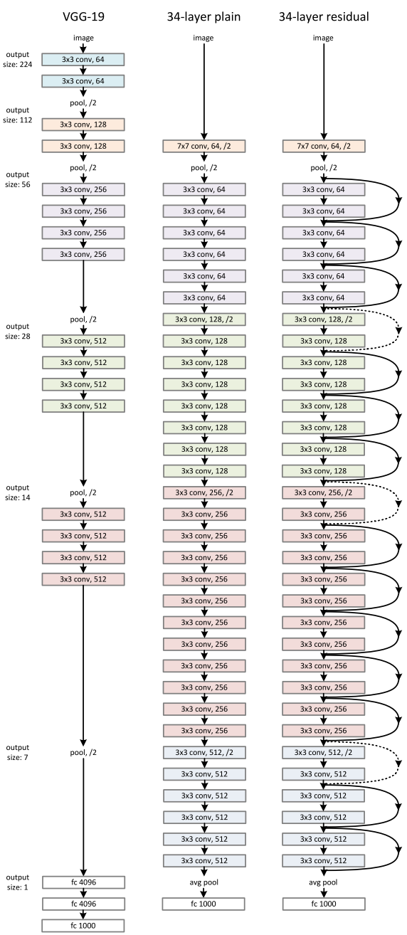
After the success of AlexNet at the ILSVRC in 2012, the top preforming algorithms were dominated by convolutional neural networks. In 2014, a team from Google submitted a CNN that reduced the error rate to under 7%. In the same year, a runner up team of Karen Simonyan, Andrew Zisserman submitted VGG. In the ILSVRC, VGG19, the architecture that was used in this project, earned an error rate of 9%. Moreover, it accomplished this while boasting an extremely simple architecture of only 3x3 convolutional layers stacked on top of each other. The VGG is shown below.
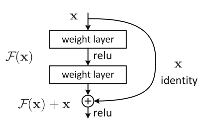
At ILSVRC 2015, Kaiming He, Xiangyu Zhang, Shaoqing Ren, and Jian Sun introduced a Residual Neural Network (ResNet). ResNet was unique due "residual blocks" (shown above), which allowed one or more layers to be skipped. During the 2015 ImageNet Large Scale Visual Recognition Competition, ResNet achieved a top-5 error rate of 3.57%. An architecture comparison of VGG and ResNet is shown below.
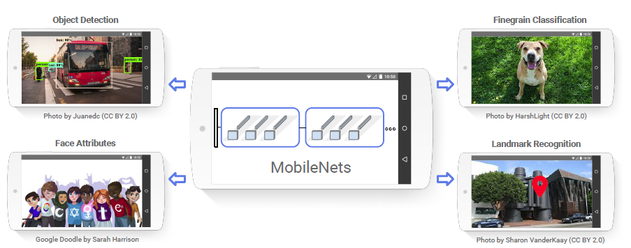
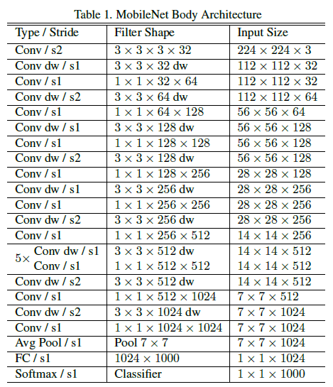
As CNN's gained popularity, researchers aimed to make them faster and lighter. One such CNN, MobileNet, emerged as a particularly effective architecture. MobileNet utilizes depthwise seperable convolutions to greatly reduce the number of parameters while retaining the same depth levels as "normal" CNN's. The resulting performance gains make MobileNet a great choice for computer vision on devices with less power, such as cellphones and embedded cameras. MobileNet V1's architecture is shown below.
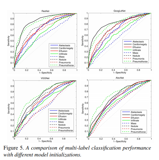
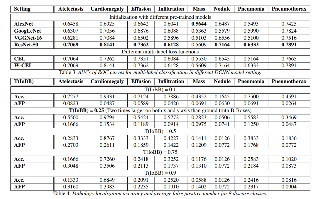
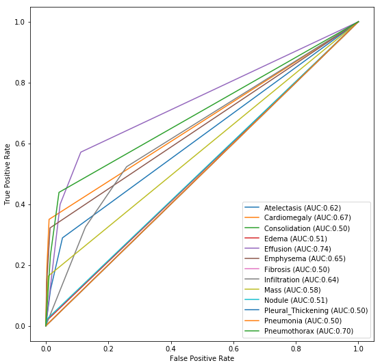
This dataset was gathered by the NIH and contains over 100,000 anonymized chest x-ray images from more than 30,000 patients. The results shown below are taken from Wang et. al.
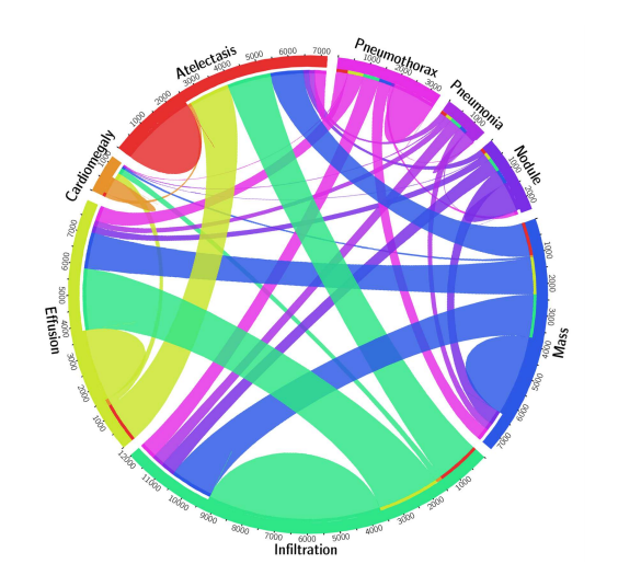
The image set involves diagnoses that were scraped from radiology reports and is a multi-label classification problem. The diagram below shows the proportion of images with multi-labels in each of the 8 pathology classes and the labels' co-occurrence statistics.
Comparison of multi-label classification performance with different model architectures.
Tabulated multi-label classification performance with best results highlighted.
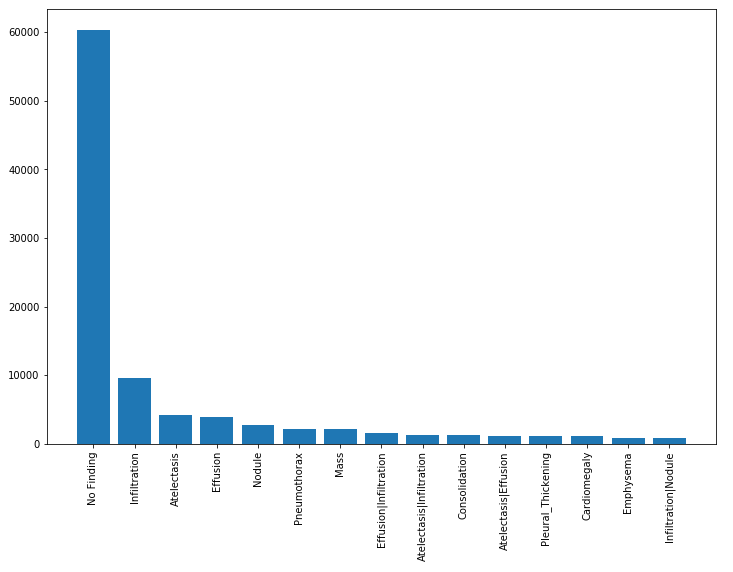
The figure below shows the distribution of findings from the diagnoses tied to the x-rays. Here we see that 60,000 x-rays had no finding. Therefore, for the purpose of our classification problem, we discard these results.
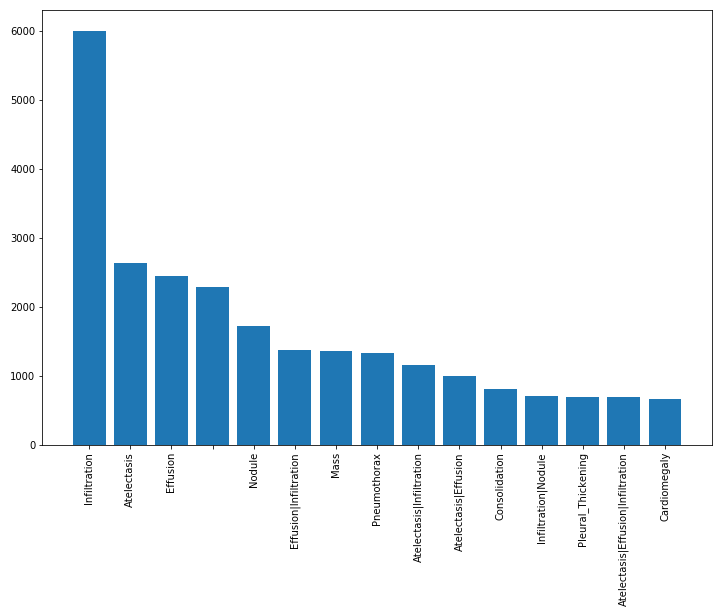
Further, because neural networks rely upon large training sets, we discard any rare diagnoses, that is, we eliminate those with fewer than 1000 occurrences. The resulting distribution of diagnoses is shown below.
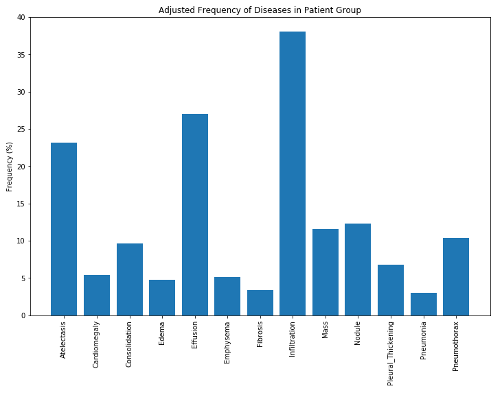
Finally, in order to better understand the distribution of results, we can observe relative frequency to see which diagnoses are most common.
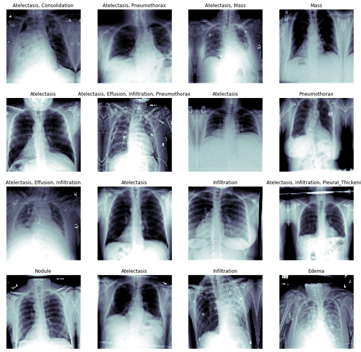
Below are sample images that show different labeled types of diagnoses along with their chest x-ray images.
While it appears that Adagrad, and adadelt may reach convergence faster, there is no substantially different loss as a result of optimizer selection. When this function was run with larger numbers of training examples per epoch, adam outperformed (graphic not shown). Based on the results shown in the figure above, we can accept the use of adam based on this particular dataset.
Code for Batch Size and Learning Rate Determination
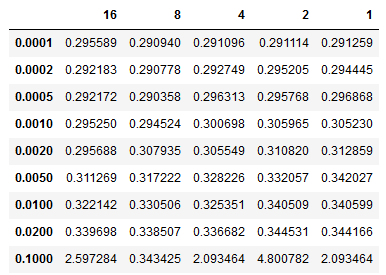
The table below shows batch size accumulation steps (32 x n) vs learning rate. We can see that our model achieves better loss for learning rates around 0.0005 and with a gradient accumulation step size of 8 or batch size of 256. We observed similar performance for batches both smaller and larger, so we can be confident that batch sizes of 1024, or 2048 would not yield substantially improved performance. Going forward we can use the ADAM optimizer along with a batch size of 256 using gradient accumulation.
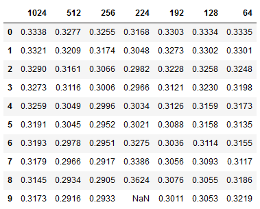
The above table shows image size resolution. Mobile net was designed for (224 x 224). VGG19 was also designed with a native resolution of (224 x 224). However, inceptionV3 1111111111111111111 was designed with a resolution of (299 x 299). We might expect no improvement in performance beyond the initial design of the network. However, model performance will be dependent upon the particular data set that is being used. We do in fact see the best performance with images of size (512 x 512). While in comparison, (224 x 224) appears to over-train and result in decreasing performance with validation loss. Intuitively, we also observe that low resolution images such as (64 x 64) have strictly worse performance.
Therefore, we will go forward with a resolution of (512 x 512), knowing with confidence that we should get results at least as good as using the native resolution of the various models (299 x 299).
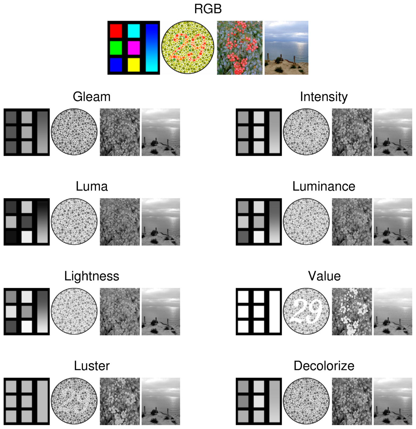
Initially we trained the model making use of grayscale images, as X-ray medical images can typically be inferred to not have significant information present in the color channels. However, this is an assumption that we also test. Kanan and Cottrell show that the information present in RGB channels and the algorithm used to produce grayscale can be meaningful.
Because grayscale images utilize only a single channel while RGB uses 3 channels, with grayscale we can fit more images in memory and run larger batch sizes. However, we may be sacrificing model performance by losing information. As an experiment, a comparison was made between RGB and grayscale images for two different image sizes. From the figure below we see negligible performance difference between RGB and grayscale. For the sake of conservatism, because we are running our model on a V100, we have enough memory that we can use RGB and know that we will get at worst, the same performance as with grayscale.
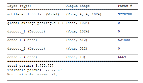
Below we can see the results from our initial simple model created in Keras after tuning the various hyper-parameters. We make use of the mobilenet and add dense layers with a final sigmoid activation for classification prediction.
From this model, we can see that not all diagnoses have the same levels of predictive power. For instance, we can see that we can predict the presence of Edema much more readily than pneumonia. In fact, at this point we have outperformed the model across almost all of the identified diagnoses classes. At this point, we will now see how much further improvement we can achieve with other model architectures.
Code for Model Architecture Determination
In order to determine which model performs best, we ran a series of experiments. We trained a selection of models with a few dense layers at the bottom of the network to predict our binarized classes.
- Mobilenet
- Mobilenet V2
- Inception Resnet V2
- Inception V3
- VGG19
- NASNet
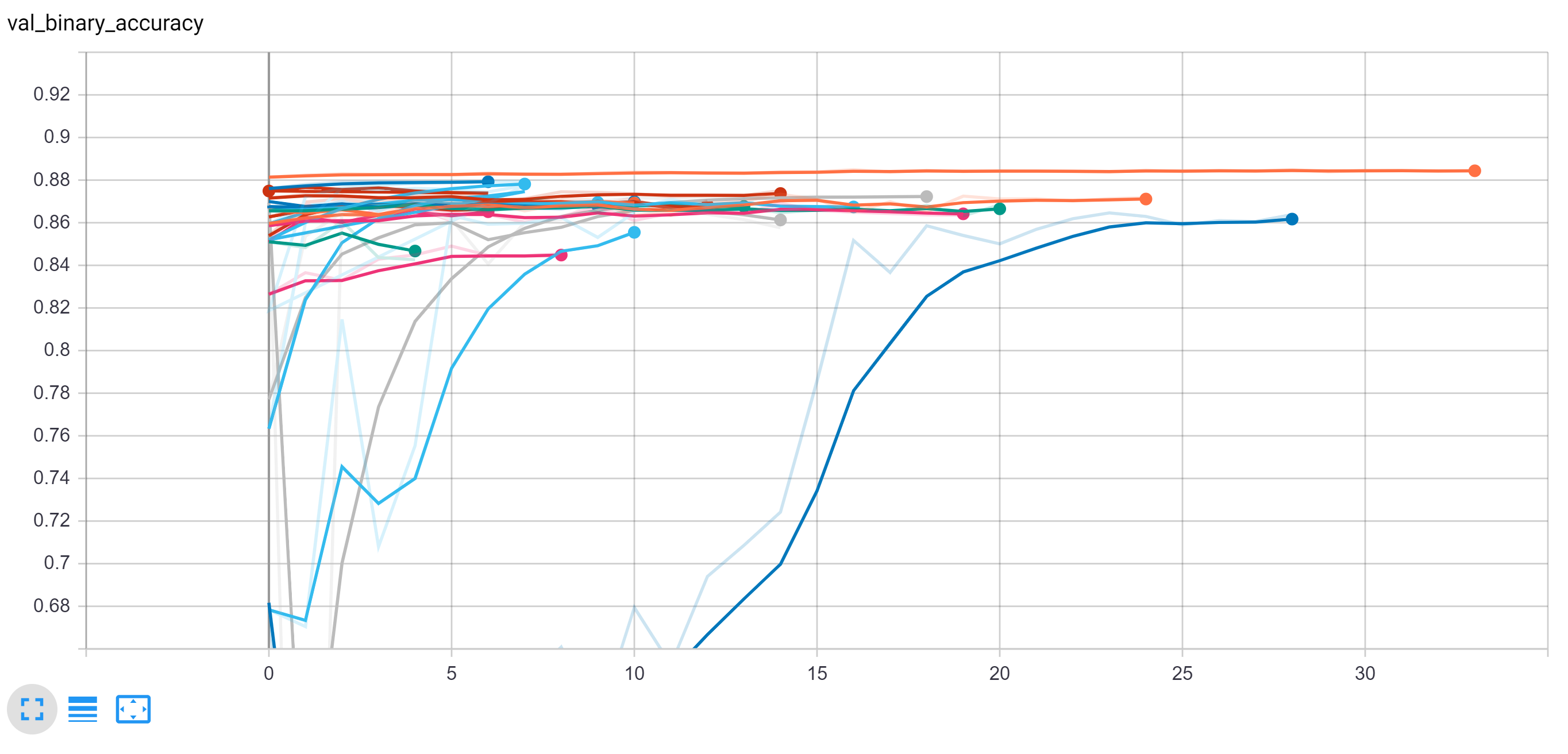
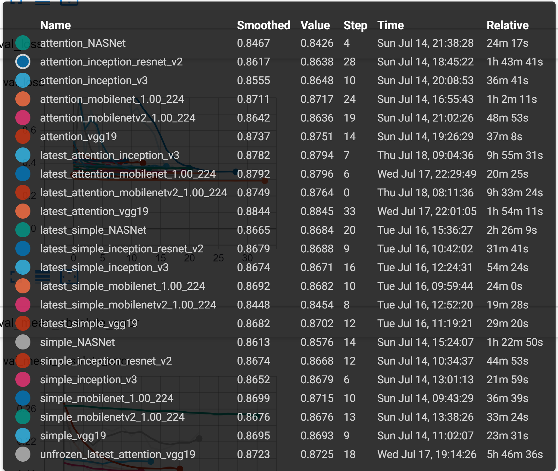
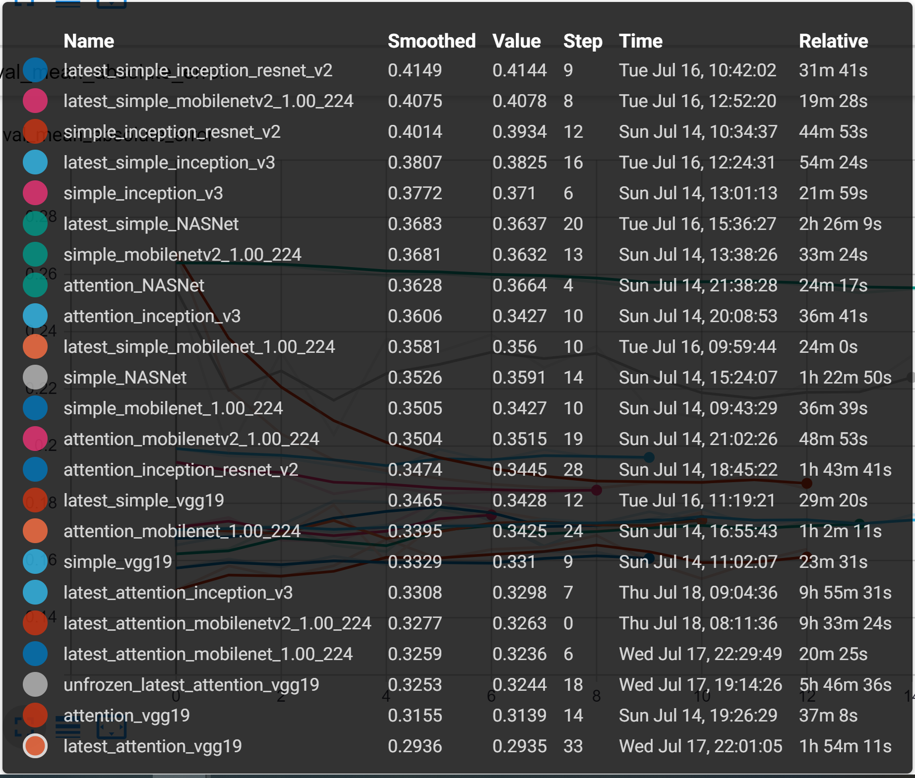
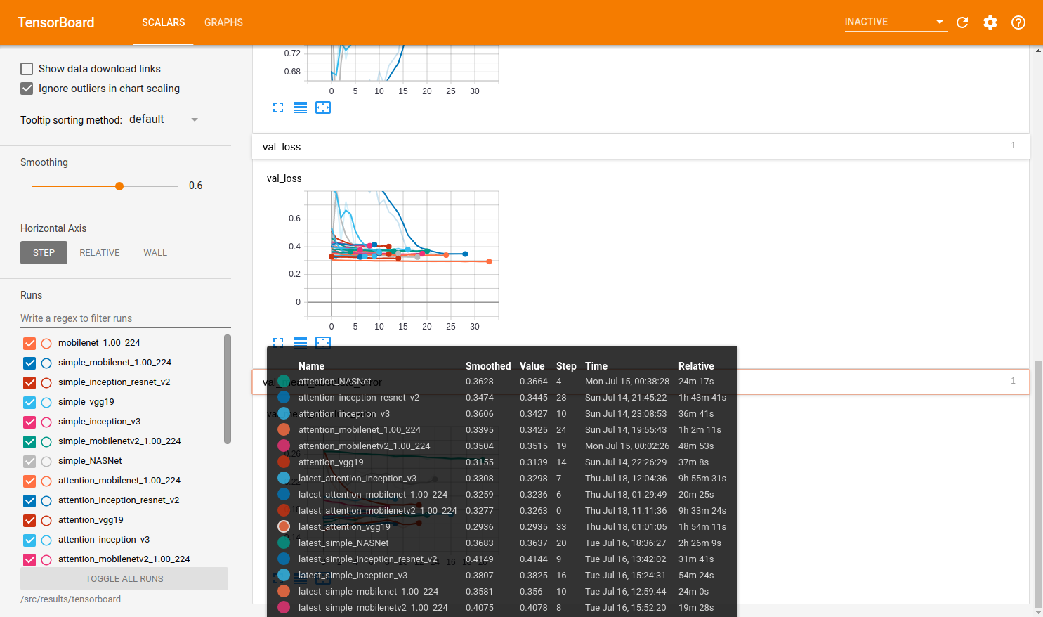
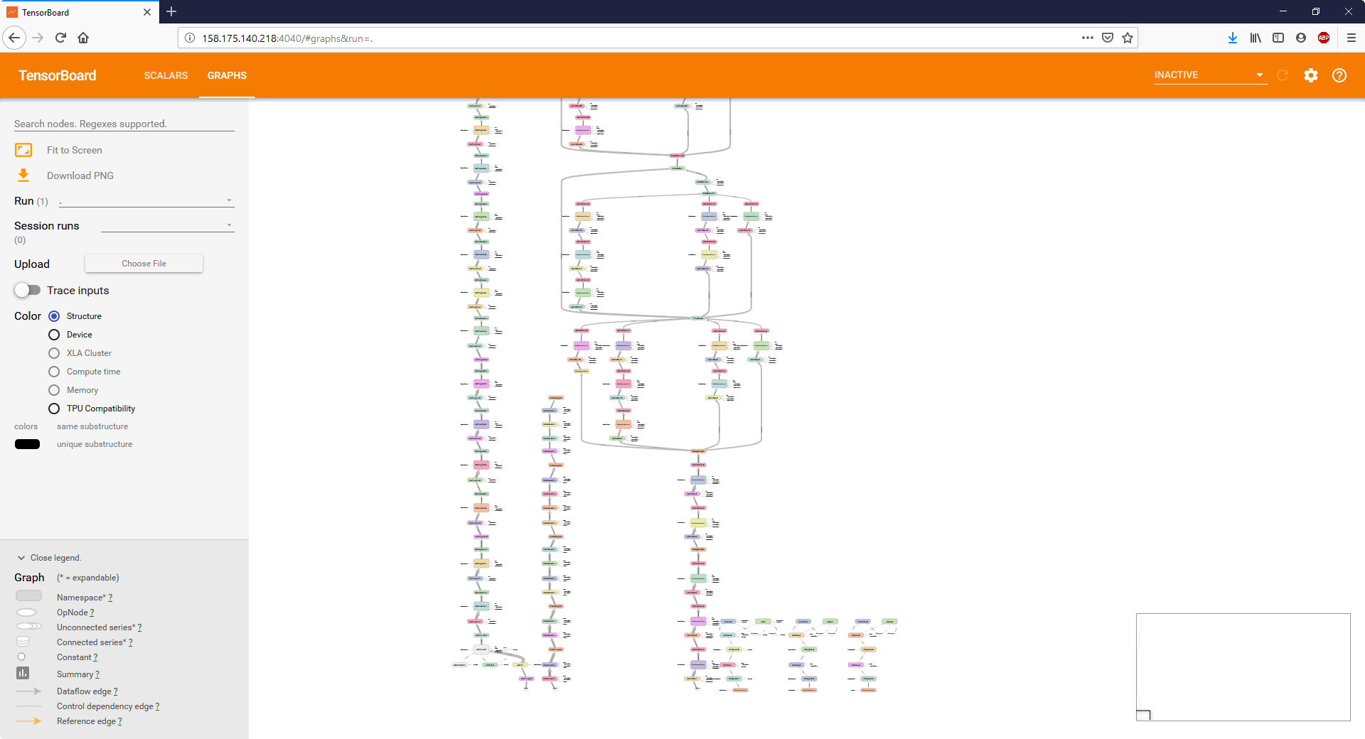
These results as well as the final results are all displayed together on the following two tensorboard outputs. From this experimentation, we were able to determine that many of these models ultimately perform very similarly in terms of accuracy to one another when fully trained but with minor differences.
Note below the total training time each network required to converge. Most networks quickly reached a good accuracy and had very small improvement over the epochs
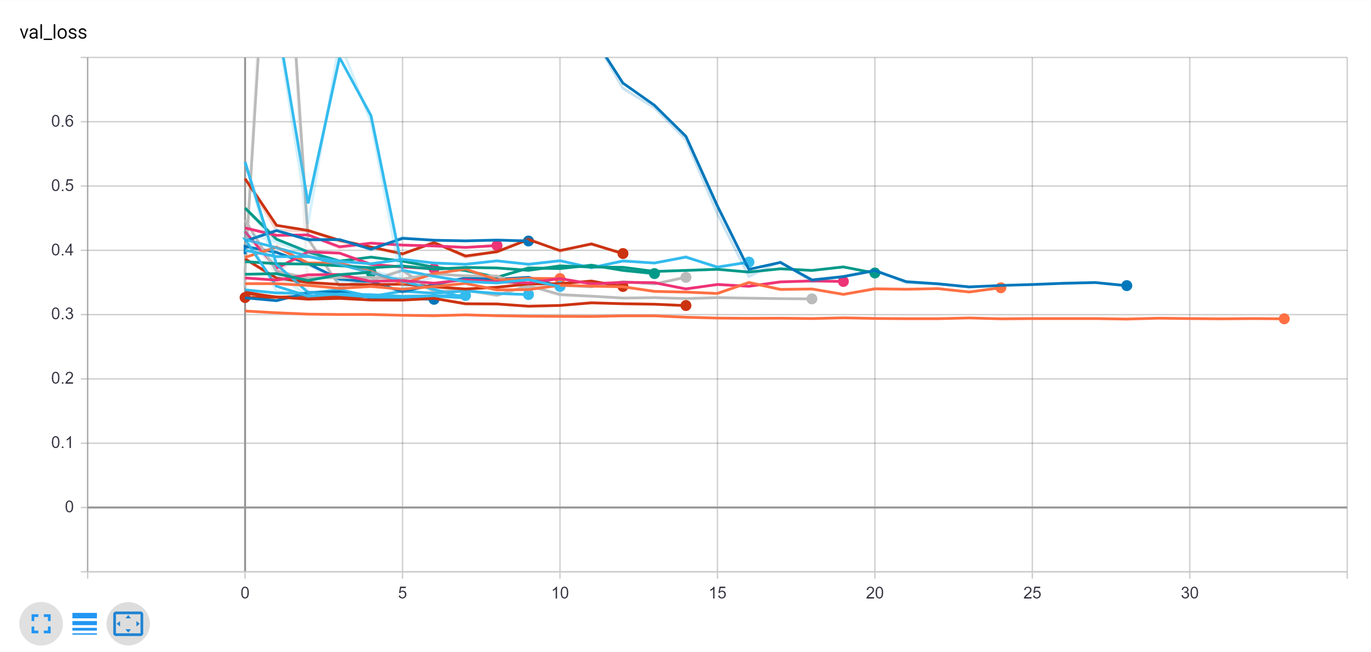
However, as can be seen on the comparison of validation loss, some of the models do outperform.
Note: VGG generally outperformed the other networks in this training collection and the VGG with the attention network improved the simple VGG, increasing the training time more than threefold
We can attempt to improve our model through the use of an attention layer. The attention layer localizes the region of the image that is strongly activating the specific classes, in this case, a particular diagnosis. This can improve the performance of the network as well as ultimately aid in the interoperability of our model by visualizing the attention layer as shown below in the following figures.
We can see that for a given network we boosted the binary accuracy by approximately 2% with the inclusion of the attention layer when compared with the frozen network.
Here we present a few high confidence examples along with their attention maps.
One notable example here is the fifth from the top and the very precise small attention region of the corresponding attention map.
The next picture is a similar plot of random high confidence examples. We demonstrate here the importance that the the attention layer adds to the interpretability of the predictions: In the last example, although we got a very confident prediction, we see that the network actually paid attention to the top left corner, which is effectively outside the X-ray, rendering this prediction a possible false positive.
As can be seen on the comparison of validation loss, our best results should be determined with the use of VGG19, Inception V3, Mobilenet, and MobilenetV2 all with attention.
We can then use these fully trained models for inference or ensemble them together to attempt to improve performance.
We are able to take our best performing networks and create an ensemble from the inferred predicted classes. There are a number of different ensemble methodologies that were explored. It is possible to perform any of the following operations:
- Simple Averaging of predictions
- Weighted Average of predictions
- Hard Vote where values are coerced into binary then voted
- Max Vote where the value with the highest predicted value is always selected
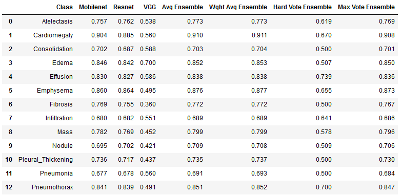
As can be seen in the table below, we were able to improve the performance of the model with the implementation of an ensemble.
The hard vote ensemble is interesting, because although it results in less overall accuracy, the model has an exceptionally low false negative rate. Such an ensemble could be of use particularly in this circumstance where positive classes found with hard voting should be taken much more seriously.
Code for Inference on TX2 in a Jupyter Notebook
After the models are fully trained on a powerful machine, in this case, a V100 on the ibmcloud, we may ultimately want to use the models on an internet of things (IOT) device. This could be extremely useful for applications where interpretation of an X-ray is not easily possible, for instance in a 3rd world country, or a field application such as in the military.
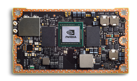
This project utilizes NVIDIA TX2 for runtime inference. These are mobile devices with reasonably powerful GPUs onboard. Because there is limited GPU RAM, we will have to use much smaller batch sizes.
We converted the codebase and containerized the process to easily build and distribute this functionality. This code base supports both jupyter notebook or command line inference. For ease of use, shell scripts are used to start and end the container.
Execution of the docker commands is shown below:
docker run \
--name tensorflow \
--privileged \
-v "$PWD":/content/project \
-v "/media/brent/data":/content/data \
-p 8888:8888 \
--rm \
-ti tensorflow_tx2 \
jupyter notebook --no-browser --port 8888 --ip=0.0.0.0 --allow-root --NotebookApp.token='root' --notebook-dir=/content/
docker run \
--name tensorflow \
--privileged \
-v "$PWD":/content/project \
-v "/media/brent/data":/content/data \
-p 8888:8888 \
--rm \
-ti tensorflow_tx2 \
/bin/sh -c 'cd content/project; python3 ./inference.py'
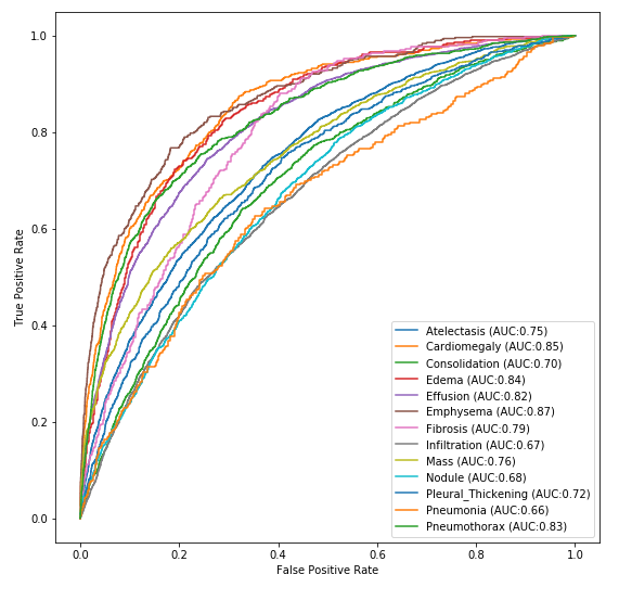
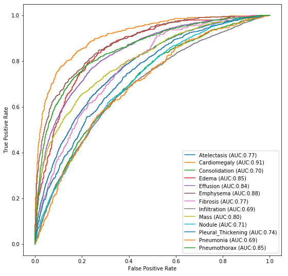
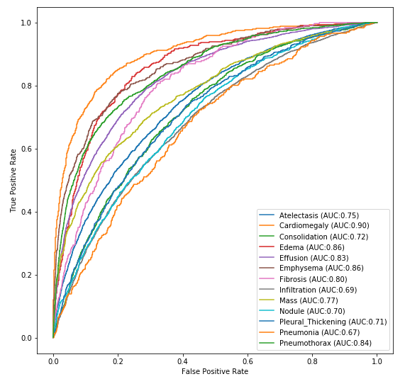
For simplicity and performance, we utilized the mobilenet architecture. The trained weights are lightweight (15MB) and the model can easily fit on many IOT device GPUs. Below is the ROC graph from runtime inference.
We were ultimately able to achieve binary classification performance of over 88% on the total dataset. Below we compare our table of results next to the published results from 2017. As can be seen, advances in neural networks have allowed us to easily surpass the published results across all categories.
If using AWS, as assumed by these setup instructions, provision an Ubuntu 18.04 p2.xlarge instance. It's got older GPUs (Tesla K80) but is much cheaper. Make sure to upgrade the storage space (e.g. 500 GB). Also, make sure to pick a prebuilt Deep Learning AMI during the first step of the provisioning process. The most current version as of writing is Deep Learning AMI (Ubuntu) Version 23.0 - ami-058f26d848e91a4e8. This will already have docker and nvidia-docker pre-installed and will save you a lot of manual installation "fun".
Provision a server to run the training code. You can you this server as your development environment too.
Install the CLI, add your ssh public key, and get the key id
curl -fsSL https://clis.ng.bluemix.net/install/linux | sh
ibmcloud login
ibmcloud sl security sshkey-add LapKey --in-file ~/.ssh/id_rsa.pub
ibmcloud sl security sshkey-list
Provision a V100 using this key id
ibmcloud sl vs create \
    --datacenter=wdc07 \
    --hostname=v100a \
    --domain=your.domain.com \
    --image=2263543 \
    --billing=hourly \
    --network 1000 \
    --key={YOUR_KEY_ID} \
    --flavor AC2_8X60X100 --san
Wait for the provisioning completion
watch ibmcloud sl vs list
SSH on this host to setup the container.
ssh -i ~/.ssh/id_rsa {SERVER_IP}
Note:You'll need to check-in your public SSH key in the keys folder and modify the last layer of the dockerfile to get access to the container from VsCode
Need to Add 2 TB secondary Hard-drive to Device via softlayer device list portal.
If you haven't already, clone the project Git repository to your instance. Doing so in your home directory is convenient, and this document assumes you have done so.
cd ~
git clone https://github.com/paloukari/NIH-Chest-X-rays-Classification
Downloading and inflating the data, and building the development container has been automated in the setup.sh script.
cd ~/NIH-Chest-X-rays-Classification
chmod +x setup.sh
./setup.sh {YOUR_KAGGLE_ID} {YOUR_KAGGLE_KEY}
Note: Get your Kaggle credentials from the Kaggle account page -> Create New API Token. This is needed to download the data.
Run the chest_x_rays_dev Docker container with the following args.
NOTE: update the host volume mappings (i.e.
~/NIH-Chest-X-rays-Classification) as appropriate for your machine in the following script:
sudo docker run \
    --rm \
    --runtime=nvidia \
    --name chest_x_rays_dev \
    -ti \
    -e JUPYTER_ENABLE_LAB=yes \
    -v ~/NIH-Chest-X-rays-Classification:/src \
    -v /data:/src/data \
    -p 8888:8888 \
    -p 4040:4040 \
    -p 32001:22 \
    chest_x_rays_dev
You will see it listed as chest_x_rays_dev when you run docker ps -a.
Note: in the container, run
service ssh restart, sometimes this is needed too to update the ssh settings.
Once inside the container, try running:
nvidia-smi
If it was successful, you should see a Keras model summary.
After you've started the container as described above, if you want to also open a Jupyter notebook (e.g. for development/debugging), issue this command:
Inside the container bash, run :
jupyter lab --allow-root --port=8888 --ip=0.0.0.0
Then go to your browser and enter:
http://127.0.0.1:8888?token=<whatever token got displayed in the logs>
We need to setup the container to allow the same SSH public key. The entire section could be automated in the dockerfile. We can add our public keys in the repo and pre-authorize us at docker build.
To create a new key in Windows, run:
Powershell:
Add-WindowsCapability -Online -Name OpenSSH.Client~~~~0.0.1.0
ssh-keygen -t rsa -b 4096
The key will be created here: %USERPROFILE%.ssh
Inside the container, set the root password. We need this to copy the dev ssh pub key.
passwd root
Install SSH server
apt-get install openssh-server
systemctl enable ssh
Configure password login
vim /etc/ssh/sshd_config
Change these lines of /etc/ssh/sshd_config:
PasswordAuthentication yes
PermitRootLogin yes
Start the service
service ssh start
Now, you should be able to login from your dev environment using the password.
ssh root@{SERVER_IP} -p 32001
To add the ssh pub key in the container, from the dev environment run:
SET REMOTEHOST=root@{SERVER_IP}:32001
scp %USERPROFILE%\.ssh\id_rsa.pub %REMOTEHOST%:~/tmp.pub
ssh %REMOTEHOST% "mkdir -p ~/.ssh && chmod 700 ~/.ssh && cat /tmp/tmp.pub >> ~/.ssh/authorized_keys && chmod 600 ~/.ssh/authorized_keys && rm -f /tmp/tmp.pub"
Test it works:
ssh -i ~/.ssh/id_rsa {SERVER_IP} -p 32001
Now, you can remove the password root access if you want.
In VsCode, install the Remote SSH extension. Hit F1 and run VsCode SSH Config and enter
Host V100
    User root
    HostName {SERVER_IP}
    Port 32001
    IdentityFile ~/.ssh/id_rsa
Hit F1 and select Remote-SSH:Connect to Host
Once in there, open the NIH-Chest-X-rays-Classification folder, install the Python extension on the container (from the Vs Code extensions), select the python interpreter and start debugging.
The model is trained through train.py. The configuration of the models can be changed with a number of helper functions and parameters that are set in params.py.
To train a single model with mobilenet run the train() function in train.py.
To visualize results using tensorboard, use the terminal:
tensorboard --logdir=/src/results/tensorboard/single_model/ --port=4040
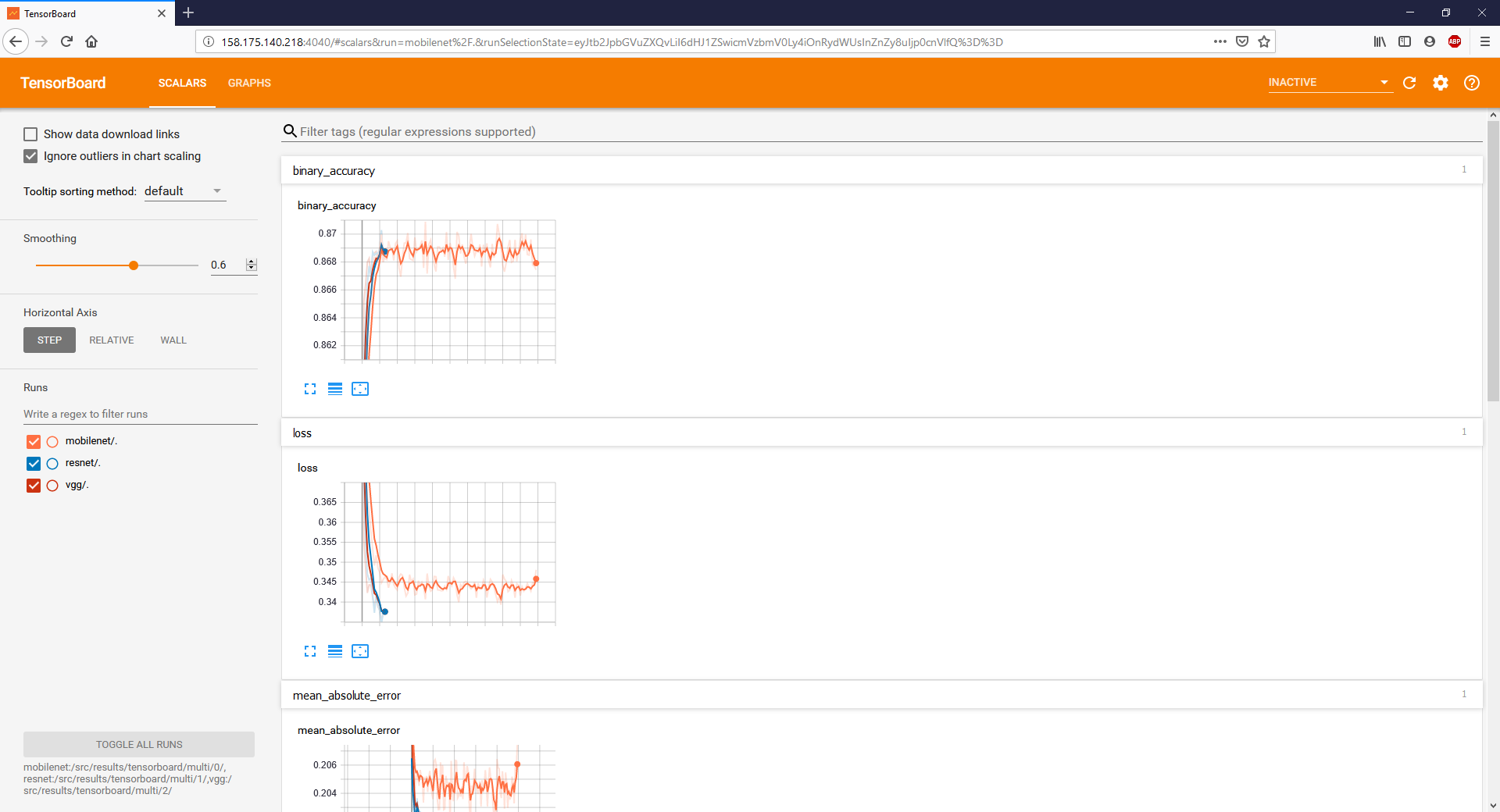
To train multiple models for comparison between mobilenet, VGG, and ResNet run the train_simple_multi() function in train.py.
To visualize results using tensorboard, use the terminal with paths to the models:
tensorboard --logdir=mobilenet:/src/results/tensorboard/multi/0/,resnet:/src/results/tensorboard/multi/1/,vgg:/src/results/tensorboard/multi/2/ --port=4040
-
Wang X, Peng Y, Lu L, Lu Z, Bagheri M, Summers RM. ChestX-ray8: Hospital-scale Chest X-ray Database and Benchmarks on Weakly-Supervised Classification and Localization of Common Thorax Diseases. ChestX-ray8: Hospital-scale Chest X-ray Database and Benchmarks on Weakly-Supervised Classification and Localization of Common Thorax Diseases.
-
NIH News release: NIH Clinical Center provides one of the largest publicly available chest x-ray datasets to scientific community. Original source files and documents: https://nihcc.app.box.com/v/ChestXray-NIHCC/folder/36938765345
-
Kanan C, Cottrell GW (2012) Color-to-Grayscale: Does the Method Matter in Image Recognition? PLoS ONE 7(1): e29740. https://doi.org/10.1371/journal.pone.0029740
-
Skymind. "A Beginner's Guide to Attention Mechanisms and Memory Networks". https://skymind.ai/wiki/attention-mechanism-memory-network
