Estimate Stain Index for single stained cytometry files.
To install the latest version of the package, run the following R commands
install.packages("devtools")
devtools::install_github("Saeyslab/CytoBright")
For the example, we load some data that is stored inside the CytoBright package. You should adapt this directory to point to your directory of interest. While the metadata table can also be a dataframe created in R, it is often easiest to store this information in an excel file.
Important values in the excel file:
| Fluorochrome | Detector | File |
|---|---|---|
| BUV395 | UV379-A | UV laser_BUV395.fcs |
| BV421 | V431-A | V laser_BV421.fcs |
| FITC | B530-A | B laser_FITC.fcs |
| PE | YG586-A | YG laser_PE.fcs |
| AF700 | R730-A | R laser_AF700.fcs |
fcs_dir <- system.file("extdata/example_data/with_unstained",
                       package = "CytoBright")
meta <- readxl::read_xlsx(file.path(fcs_dir,
                                    "220309-FlowCore-SymphonyA3-CD4.xlsx"))
meta <- as.data.frame(meta, check.names = FALSE)
Update the meta dataframe to contain consistent fluorochrome names, full file paths and unique IDs. As in this case every fluorochrome occurs only once, we can use the flurochrome name as the ID.
meta$Fluorochrome <- clean_fluorochromes(meta$Fluorochrome)
meta$File <- file.path(fcs_dir, meta$File) # Add directory
meta$ID <- rownames(meta) <- meta$Fluorochrome
Our package also contains a table of some theoretical brightness values, as derived from different company websites.
expected_brightness <- theoretical_brightness()
meta$BrightnessLevel <- expected_brightness[meta$Fluorochrome, "Brightness"]
We will also apply some pregating to only work on events of interest.
This gating information is stored in a list of lists structure, to allow
multiple consecutive gating steps. Each gating step should be described by a
list which corresponds with the arguments for the estimate_gate function,
of which the marker_values argument is of main interest, giving estimates
for the gate boundaries. flowDensity::deGate is used to try to find a possible
cutoff in the range of e.g. the minimal value plus or minus the range_min.
If no value is found in that range, the specified minimal value will be taken
instead.
gating_info <- list(list(marker_values = list(`FSC-A` = c(min = 60000,
                                                          range_min = 50000,
                                                          max = 125000,
                                                          range_max = 50000),
                                              `SSC-A` = c(max = 80000,
                                                          range_max = 50000))))
In combination with the pregating, the package also supports several additional preprocessing steps, such as removal of margins or doublets with the PeacoQC package. If pregating is performed on some fluorescent channels, a transformList might need to be passed along as well. Once we have all this information, we can estimate the brightness. In this example, we use an unstained file to estimate the negative population. If the unstained parameter is set to NULL, the negative population is taken from the single stain file itself.
brightness <- estimate_brightness(meta,
                                  preprocessing_parameters = list(compensate = FALSE,
                                                                  removeMargins = TRUE,
                                                                  removeDoublets = TRUE,
                                                                  pregate = gating_info,
                                                                  pregate_tf = FALSE),
                                  return_cells = TRUE,
                                  seed = 1,
                                  comp = NULL,
                                  unstained = file.path(fcs_dir, "Specimen_001_US.fcs"))
brightness$SI will contain all information from the original metadata,
as well as added columns for the Cutoff value determined, the MFIs of the
positive and negative populations, the range of the negative population
(0.05 and 0.95 quantiles are used), the robust Standard Deviation calculated as
(max_neg - min_neg) / 3.29, and the estimated Stain Index (SI).
This information can easily be stored in an excel file.
writexl::write_xlsx(brightness$SI,
                    "brightness_220309_SymphonyA3.xlsx")
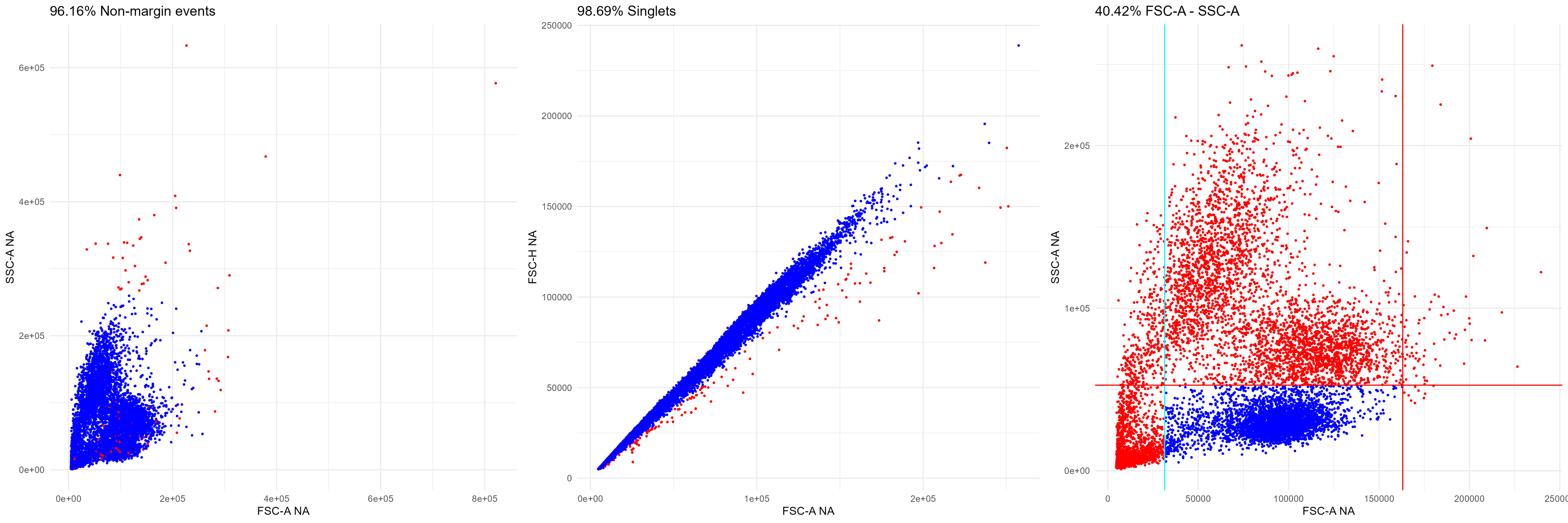
Additionally, all preprocessing figures are stored as well as some values of individual cells for visualisation purposes. They can for example be stored with the following command
ggplot2::ggsave("preprocessing_BUV395.png",
                ggpubr::ggarrange(plotlist = brightness$pregating_plots$BUV395,
                                  nrow = 1),
                width = 21, height = 7)
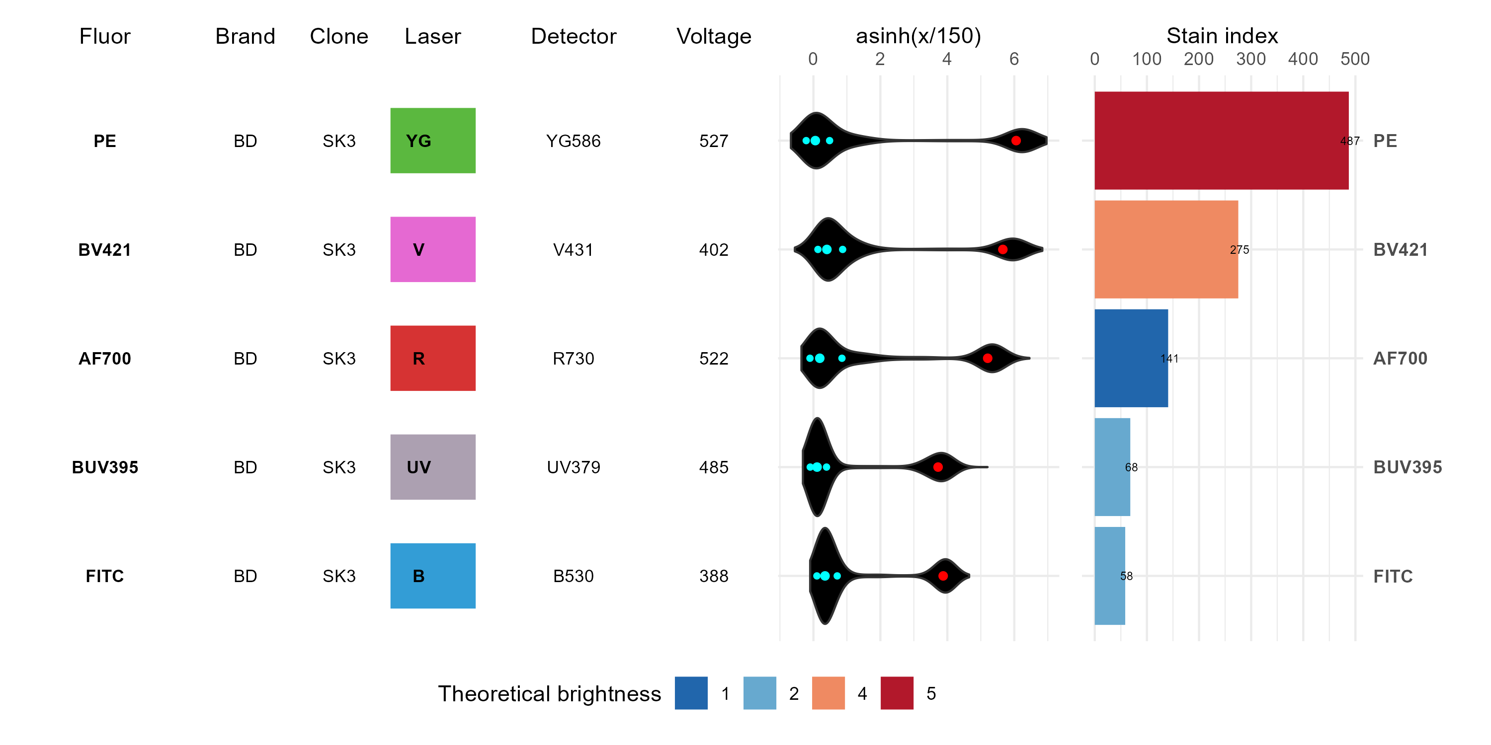
With the plot_brightness function an overview of the brightness of the
different fluorochromes can be generated.
ggplot2::ggsave("brightness_overview.png",
                plot_brightness(brightness$SI, brightness$cells),
                width = 10, height = 5)

