1) Download Python3 and pip3
2) Open Terminal
3) Run following commands
    a) sudo apt-get install python3-tk
    b) sudo pip3 install numpy
    c) sudo pip3 install mlxtend
    d) sudo pip3 install matplotlib
    e) sudo pip3 install scikit-learn
    f) sudo pip3 install sklearn-contrib-py-earth
    g) sudo pip3 install Pillow==2.2.1
4) python3 application.py in terminal
Note use pip instead of pip3 and python instead of python3 if default python version is python3 in your linux
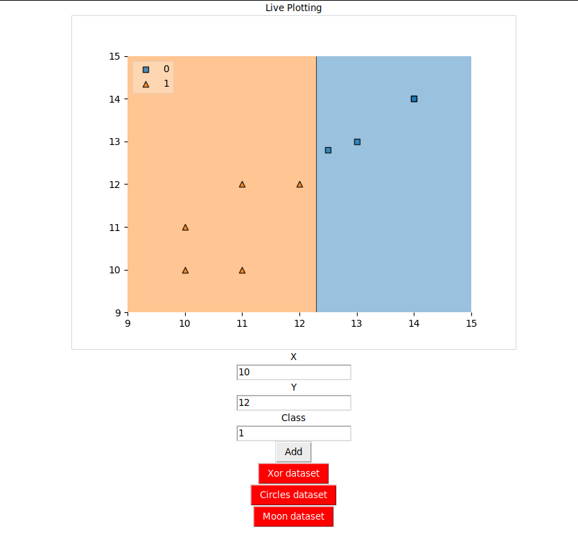
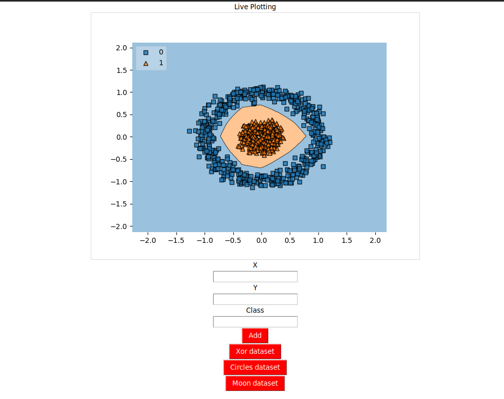
Output GUI -
By - Divyansh Verma
Subject - Machine Intelligence (MI)
Email - divyanshverma12@gmail.com
Definition - Multivariate/Multiple Adaptive Regression Splines (MARS) is a form of regression analysis which was introduced by Jerome H. Friedman in 1991. It is a stepwise linear regression algorithm. It can be defined as an attempt to modify linear models to automatically fit over non linearities in a given dataset. So in layman language it is an extension of linear models that can easily model some non linearities.
Terminology
1) Multivariate - Able to generate model based on several input variables
2) Adaptive - Generates flexible models in passes each adjusting the model
3) Regression - Estimation of relationship among independent and dependent
variables
4) Spline - A piecewise defined polynomial function that is smooth (possess high
order derivatives) where polynomial pieces connect
5) Knot - The point at which two polynomial pieces connect
Previous Methods There are various linear modeling techniques like linear regression (https://en.wikipedia.org/wiki/Linear_regression), logistic regression (https://en.wikipedia.org/wiki/Logistic_regression) etc.
They are really fast and simple algorithms and many of such linear models can be easily adapted to non linear patterns in the data by adding non-linear terms (like higher order polynomials, interaction effects or any other transformation techniques applied to original features), however to such things we should know the specific nature of the non-linearities and interactions before building such models.
There are many Data Analysis models which are naturally nonlinear and these models can be used to extract non linearity from the given dataset without detecting or identifying non-linearity in such datasets and Multivariate Adaptive Regression Spline (MARS) is one such algorithm ( Fig - 1 shows a comparison between Normal regression model and MARS model). MARS can discover non-linearities in a dataset without explicitly defining or understanding non-linearity (It will search for it).
Why to Use We need to use such non-linear regression models (MARS) as they are more flexible than linear regression models and although some non-linearity is added to the model, yet the MARS model is easy to understand and interpret and also MARS requires minimal features engineering like feature scaling or feature transformation and automatically performs features selection.
Linear Regression is the most basic regression model. Simple linear regression (SLR) assumes that statistical relationship between two continuous variables (let us say X and Y) is linear and can be defined using a simple equation: Multivariate adaptive regression splines (MARS) is an easy and simple approach to capture the non-linear relationships in the data by setting the values of knots(cutpoints) similar to step functions also known as hinge functions. The procedure assesses each data point for each predictor as a knot and creates a linear regression model with the candidate feature(s).
Example/Overview of working of algorithm - Consider a non-linear, non-monotonic dataset where Y = f ( X ). I. Look for the single point across the range of X values where 2 different linear relationships between Y and X achieve smallest error or loss. II. The result of such finding is known as hinge which is given by h ( x − a ) where a is the cut-point value. As shown in Fig - 4(A) our hinge function is h ( x − 1. 18 )such that out two linear model for Y will be - Y = β 0 +β 1 ( 1. 18 − x ) when x < 1. 18 Y = β 0 +β 1 ( x − 1. 18 ) when x > 1. 18 III. Once the first knot is found, algorithm will continue to find 2nd knot which in the given figure fig - 4(B) is x = 4.89 so, Y = β 0 +β 1 ( 1. 18 − x ) when x < 1. 18 Y = β 0 +β 1 ( x − 1. 18 ) when x > 1. 18 and x < 4. 89 Y = β 0 +β 1 ( 4. 89 − x ) when x > 4. 89 IV. Step III. continuous as long as many cutpoints(knots) are found, resulting in a good non-linear prediction equation.
Generalization
MARS Model Building Procedure
- Gather data i.e. x input variables or data-points from the dataset with y output for each x (i.e. input variable).
- Calculate or find a set of basis functions by setting knots at observed values.
- Constraint specification i.e. number of terms in the model and maximum allowable degree of interaction.
- Forward Pass - Try out different or new hinge functions and their product combinations which decreases training error.
- Backward Pass - Fix Overfitting over the training set.
- Use of generalized cross validation technique to estimate the number of optimal terms in the MARS model.
MARS Forward Pass
- MARS starts with a model which consists of an intercept term which can be defined as the mean of the response values.
- Each step MARS adds a basis function in pairs to the model and finds a pair of basis functions that gives the maximum reduction in loss or error (i.e. sum of square error).
- Each new basis function consists of a term already in the model multiplied by a new hinge function. As define above hinge function is defined by a variable and a knot so to add a new basis function, and MARS model search over all the combination of following a. Existing terms b. All variables c. All values of each variable
- To calculate the coefficient of each term MARS applies a linear regression over the terms.
MARS Backward Pass
- Forward Pass leads to an overfitted model (An overfitted model is a model that gives good accuracy on a test dataset used to build a model but does not generalize well to new data or real world data.
- So to make a better model, pruning is used which is a major functionality of backward pass.
- It removes one term at a time from the model.
- Remove the term which increases the error or loss by minimum amount.
- Continue removing terms until cross validation is satisfied. The MARS model uses Generalized Cross Validation (GCV).
Generalized Cross Validation MARS backward pass uses generalized cross validation (GCV) for comparing the output/accuracy of model’s subsets in order to choose the best subset. GCV is a form of regularization i.e. it trades off goodness of fit against model complexity (As used in various neural network models). GCV is used to approximate the error or loss that will be there by removing one hinge function or a set of that.
There is nothing wrong in having a lot of hinge functions but a model that fits to noise in the dataset can give poor results on real world data. Assumptions No assumptions are made about the environment or distribution of data-points. The only requirement for the MARS model to perform well is that variables should not be highly correlated to one another as this can lead to difficulty in estimation.
Advantages of MARS
- Automatically detects interactions between variables.
- Fast and computationally efficient.
- Easy to handle data with high dimensions.
- Non-linear relationships are handled well.
- More Flexible than linear models.
- Simple to understand and interpret.
- Both continuous and discrete data can be handled well.
- Requires no data preparation.
- As computationally fast, can handle large datasets.
Output of MARS on a dataset Given dataset can be downloaded from this link (Dataset). When plotted the dataset distribution looks like this Research Implementation Related Papers -
- C. Briand and Bernd Freimut (2004). “Using multiple adaptive regression splines to support decision making in code inspections”. https://www.sciencedirect.com/science/article/pii/S
- De Veaux, R.D., Psichogios, D.C., Ungar, L.H., 1993. A comparison of two nonparametric estimation schemes: MARS and neural networks. Computers Chemical Engineering 17 (8), 819–837.
- Friedman, J. H. (1991). "Multivariate Adaptive Regression Splines". The Annals of Statistics . 19 (1): 1–67. CiteSeerX 10.1.1.382.970. doi:10.1214/aos/1176347963. JSTOR 2241837 . MR 1091842 . Zbl 0765.62064. http://www.stat.yale.edu/~lc436/08Spring665/Mars_Friedman_91.pdf
- Chi-Jie Lu ; Chih-Hsiang Chang ; Chien-Yu Chen ; Chih-Chou Chiu ; Tian-Shyug Lee “Stock index prediction: A comparison of MARS, BPN and SVR in an emerging market” https://ieeexplore.ieee.org/document/
- Wengang Zhang, Anthony T.C.Goh. “Multivariate adaptive regression splines and neural network models for prediction of pile drivability”. https://www.sciencedirect.com/science/article/pii/S
- Prasenjit Dey, Ajoy K.Das. “Application of Multivariate Adaptive RegressionSpline-Assisted”. https://www.sciencedirect.com/science/article/pii/S
Other Links -
- Github Repo - https://github.com/failedcoder12/MARS-Multivariate-Adaptive-Regession-Spli ne-
- Graphs - https://colab.research.google.com/drive/1G-QeE9Fcr2qOaWimspiMTQdKfUrH yktd?usp=sharing
- MARS Model - https://colab.research.google.com/drive/1sW2pCjWeoJKQ0YHLYl26kLRfTRm 1iRHV?usp=sharing
- GUI builder - https://colab.research.google.com/drive/1f8GPYn-Tz-hcKvVAw1MxOrBW55pf XDSP?usp=sharing
References
- Friedman, J. H. (1991). "Multivariate Adaptive Regression Splines". The Annals of Statistics . 19 (1): 1–67. CiteSeerX 10.1.1.382.970. doi:10.1214/aos/1176347963. JSTOR 2241837 . MR 1091842 . Zbl 0765.62064.
- https://bradleyboehmke.github.io/HOML/mars.html#final-thoughts-
- http://www.ideal.ece.utexas.edu/courses/ee380l_ese/2013/mars.pdf
- https://support.bccvl.org.au/support/solutions/articles/6000118097-multivariate -adaptive-regression-splines
- Milborrow S (2015) Notes on the earth package. http://www.milbo.org/doc/earth-notes.pdf
- Trevor Hastie, Stephen Milborrow. Derived from mda:mars by, and Rob Tibshirani. Uses Alan Miller’s Fortran utilities with Thomas Lumley’s leaps wrapper. 2019. Earth: Multivariate Adaptive Regression Splines . https://CRAN.R-project.org/package=earth.
- http://media.salford-systems.com/library/MARS_V2_JHF_LCS-108.pdf
- Multivariate Adaptive Regression Splines. Wikipedia. http://en.wikipedia.org/wiki/Multivariate_adaptive_regression_splines
- M. Nash and D. Bradford. Parametric and Nonparametric Logistic Regressions for Prediction of Presence/Absence of an Amphibian. EPA Oct. 2001. http:// www.epa.gov/esd/land-sci/pdf/008leb02.pdf.
- The Elements of Statistical Learning (2nd ed.). Springer, 2009. http://www-stat.stanford.edu/~hastie/pub.htm. 11.Tklnter - https://wiki.python.org/moin/TkInter 12.Mlxtend-http://rasbt.github.io/mlxtend/user_guide/plotting/plot_decision_region s/ 13.GUI Creation - How to create a real-time plot with matplotlib and Tkinter 14.Pyearth library - https://pypi.org/project/sklearn-contrib-py-earth/ 15.Pyearth documentation - https://contrib.scikit-learn.org/py-earth/