EUBOPA

European Basket Option Pricing Approaches

EUBOPA
GOAL 1
Goal 2
- Comparison between Neural Network and Monte Carlo Numerical Method
Goal 3

Scope

This project is designed to fulfil the assessment requirements for the Machine Learning Engineer post at Multiverse Computing.

Objective

The objective of this assessment task is to develop three different approaches from three mathematical domains that can be used to value a stock option and then compare the results.

Problem Statement

The client wants to explore novel methodologies for accelerating the pricing of exotic derivatives. A neural network is to be designed for pricing the European Basket options under Black-Scholes assumptions. Once done, the prices predicted by the trained model are to be compared with a traditional numerical solver for option pricing. Lastly, the results of both the strategies are to be compared against an analytical solution for a single asset.

Definitions of Financial References

Black-Scholes Formula

This is a globally acceptable model of Quantitative Finance to price the derivatives under some fixed assumptions. This formula provides a closed-form solution to the price of an option hence making it analytical in nature.
Black_Scholes Assumptions
1. Markets are fair. No transcation costs and no hiccups.
2. The under-lying asset follows the log-normal distribution.
3. Volatility and Risk-Free interest rate are constant and known.
4. This is valid only for European options which can only be exercised on the expiration date.
5. No dividends are paid out during the life of the option.
The above assumptions are also valid for the implementation of this project
geomteric Brownian Motion (gBM)

A mathematical model that is used to predict the future paths of an under-lying asset given that asset is following a Brownian Motion. In simple terms, this model helps predict the random walk of a stock price.
Monte Carlo Method

This is a numerical method that is used to foresee the life of an asset or a stock that is following a gBM.
Europan Basket Option

Basket options are based on more than one underlying assets which can only be exercised on the date of expiration. The payoff of a basket option is essentially the weighted average of all underlying assets.

1. Introduction

Option price prediction is the “act of determining” the buy or sell value of a stock option traded on an exchange. The successful prediction of a option price could yield significant profit. In this project, I have proposed a option pricing model using Artificial Neural Networks. This technique utilises five distinct features as the input parameters for training, and gives ‘Call Price’ for a European stock as the output.

2. Data set

The requirement was to design a model for the pricing of an European Basket Option. After a lot of research, I found a raw data of stock options on Kaggle.

2.1. Data set Description

There was no metadata attached to this dataset. I found following information while exploring this data.

Entity | Description ------------------------------------|----------------------------------------------------------------- Total observations in the data | 62795 Total trade symbols in the data | 2346 Highest observation in all the data | SPY (SPDR S&P 500 Trust ETF) Total Count of SPY observations | 4455

As being one of the most frequent stock in the given data, I chose to work with SPY symbol. Furthermore, I selected only the call options for the SPY dataset.

3. Assumptions attached to this project

The first assumption undertaken is that the data of SPY company is representing a weighted average of multiple underlying assets making it a basket option.
The option will only be exercised on the expiration date hence it is a European option.
Volatility, v, is calculated by the following formula.

where;

sigma is the standard deviation
N = total no. of unique days in which the trading of asset of interest happened

Using this formula, the volatility was fixed at 0.031802533217352

Adherence to the assumption no. 3 makes the whole project to be operating in the Black-Scholes world.
Risk-Free Interest Rate is set as the 10-year US treasury yield from Yahoo Finance API. At the time of data processing for this project, the risk-free interest rate was 0.012580000162125
Target variable Y for the Neural Network was set to be the Black-Scholes price of each training example. This was decided due to lack of actual trade value of the option in the primary dataset.

GOAL 1

4. ANN Model

ANNs are composed of multiple nodes, which imitate biological neurons of human brain. The neurons are connected by links and they interact with each other. The nodes can take input data and perform simple operations on the data. The result of these operations is passed to other neurons. The output at each node is called its activation or node value.Each link is associated with weight.

4.1. ANN Architecture

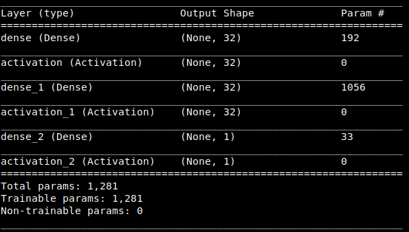
For this project, a simple ANN architecture was designed using Keras API with TensorFlow backend. Model summary is given as follows.

4.2. Input Features

Following were set at the input features to this ANN model.

Stock Price
Strike Price
Volatility
Risk Free Interest Rate
Time left in expiration

Training set is given at the following location in the repo. <root>/training/baseline.csv

4.3. Hyperparameters

For the initial model following hyperparamters were kept.

HyperParameter	Value
Loss Function	Mean Squared Error Loss
Optimizer	Adam (per-parameter adaptive learning rate)
Training Epochs	100
Train:Test:Val	70:15:15 split
Depth	2
Activation for hidden layers	Rectified Linear Unit (ReLU)
Activation of output Layer	Linear
Batch Size for last training	16

Limitations and Known Bugs

There were certain limitation that was faced at different steps while completing this assessment. I would like to mention some here.

Due to the limited background information about the Quantitative Finance domain, I spent a major section of the given time to carefully understand the actual requirement.
I didn't find a workable dataset which has the actual price of the option given in it. According to what I learned, I needed the actual price inorder to calculate the Implied Volatility of the asset so that I may then use it.
Due to time constrained assessment, I have put my core attention to figuring out the requirement. I have tried to submit a working codebase that can be used to check the understanding of the whole assessment.
Although the training loss of the network was decreased to a very considerable extent, however, the predictions and comparison was coming up quite off the mark. This is due either error-prone dataset or the incorrect implementation of volatility calculation.
Monte-Carlo implementation has an underlying assumption that the drift will always be 0.8 which is due to partial knowledged about the geometeric Brownian Motion parameters.

Code and Repository

This code should work with Python >= 3.6

Environment Setup:

pip3 install -r requirements.txt

Usage:

The main functionality of the three requirements mentioned in the assessment is implemented in runner.py file.

runner.py run in 3 modes and requires two input parameters.

--mode, -m : model used for predicting pricing
- bs: Black-Sholes model pricing
- dl: Neural-Network model based pricing
- nm: Numerical method based pricing i.e. Monte-Carlo pricing
--data, -d: accepts a file or an input from stdin
- valid json object
- data.json is given in this repo can be used to give any custom input to any specific mode

Examples

1. Black-Scholes Pricing

python runner.py -m bs -d data.json

Output:

Black-Scholes price for this European Call option = 11.308008169966485

2. Neural Network Pricing

python runner.py -m dl -d data.json

Output:

Neural network prediction price for this European Call option = 428.5238037109375

3. Monte-Carlo Pricing

python runner.py -m nm -d data.json

Output:

Monte-Carlo price for this European Call option = 784.3592326252033

EDA

Due to limited time, an extensive Exploratory Data Analysis couldn't be completed for the acquired data. However, following observation were made.

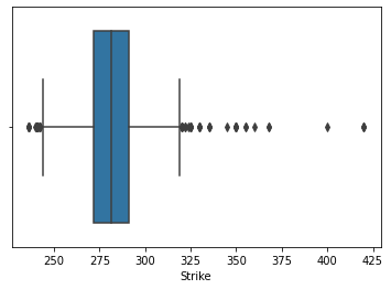
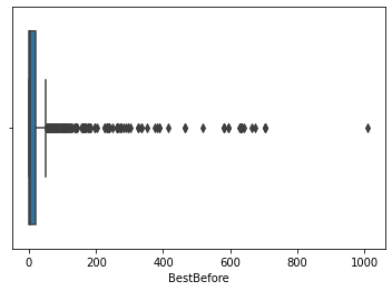
The overall distribution of the training data for SPY stock option is given below.

As we can see from the above plot that there are approx 21 observations where of strike price is quite away from the 75% quartile of the distribution, hence we need to look further into the possibility of normalizing data and handling these outliers.

As we can see from the above plot that the max value of 100+ observation of time left in expiration are aways from the from the top whisker of the box plot indicating the density of outliers in the upper and lower bounds of this variable.

Goal 2

Comparison between Neural Network and Monte Carlo Numerical Method

According to the trained model, the values of Monte Carlo and NN are not making too much sense to be reflecting any meaningful pricing. This indicates a problem with either the dataset or the volatility calculation used to set the constant.

Goal 3

Comparison of Analytical Method (Black-Scholes Pricing) vs Neural Network bs Monte Carlo Numerical Method

While looking at the results, the Black-Scholes pricing seems to be the most reasonable and correct against the NN, and Monte-Carlo method. Part of this behavior is due to the fact that Black-Scholes pricing is used as the target variable in the training of the Neural network giving it an edge of being the ground truth. Dataset, however, needs to be discussed with a domain expert.

Future Direction & Improvements

Exploratory Data Analysis of the data in hand to normalize the data for better and cleaner training.
Tabular comparison of the results from analytical, neural network and Monte Carlo approaches
Get the input data vetted by a domain expert to mitigate the inaccuracies.
Introduce Heston Volatility and then retrain the network releasing the assumption of fixed volatility.
Employ GridSearch to look for best hyper-parameter given that the input data is sound and correct.
Use LSTM network to capture the information for date of trading to learn the underlying pattern.
Better intuition of Volatility for Black-Scholes fixed v calculation to mitigate the error in current implementation.
There was a fake news release from Bloomberg on 17-07-2015 about the acquisition of Twitter for 31B USD. This happened around 11:35 am on that day. If I can get that data, I can calculate volatility as the weighted average of the X timestamp and thus can have an organic volatility for training. This will enable me to release the assumption of constant volatility from the Black-Scholes and the resulting NN implementation can have a very interesting result.
Explore the numerical methods in more detail inorder to better implement the current version.
Dataset for BitCoin and Tesla stock comparison can be scoured to study the impact of Tesla accepting and then dropping the BitCoin as their payment option thus disrupting the crypto market quite heavily a while ago.
Expand on my understanding of the quantitative finance domain to better study the market trends and nomenclature.
Keep the Learn, Try, Repeat cycle going in full swing.

sailsolar/euop

EUBOPA

Table of Contents

Scope

Objective

Problem Statement

Definitions of Financial References

Black-Scholes Formula

Black_Scholes Assumptions

geomteric Brownian Motion (gBM)

Monte Carlo Method

Europan Basket Option

1. Introduction

2. Data set

2.1. Data set Description

3. Assumptions attached to this project

GOAL 1

4. ANN Model

4.1. ANN Architecture

4.2. Input Features

4.3. Hyperparameters

Limitations and Known Bugs

Code and Repository

Environment Setup:

Usage:

Examples

1. Black-Scholes Pricing

2. Neural Network Pricing

3. Monte-Carlo Pricing

EDA

Goal 2

Comparison between Neural Network and Monte Carlo Numerical Method

Goal 3

Comparison of Analytical Method (Black-Scholes Pricing) vs Neural Network bs Monte Carlo Numerical Method

Future Direction & Improvements

References