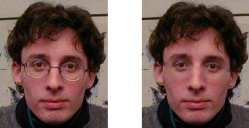
This project implements vector-valued image regularization technique using PDE's as described in the paper - Vector-Valued Image Regularization with PDEs: A Common Framework for Different Applications by David Tschumperle and Rachid Deriche
A detailed report on methods and results can be found as report.pdf. It was made as the final project for CS 663 - Digital Image Processing course in Autumn 2018 at Indian Institute of Technology (IIT) Bombay, India.
These instructions will get you a copy of the project up and running on your local machine for development and testing purposes.
- Run
/src/inpainting.mfile for image inpainting,/src/denoising.mfile for image denoising and/src/flowVisualisation.mfile for flow visualisation. - Replace the arguments of the functions with respective input image paths and set the hyperparameters you wish to use to generate the output images.
- The tuned hyperparameters for our output images can be found in
/src/main.mfile.
Figure 1: Inpainting with 21x21 neighbourhood, t=5 and 10 iterations
Figure 2: Inpainting with 10x10 neighbourhood, t=2 and 20 iterations
Figure 3: Inpainting with 20x20 neighbourhood, t=3 and 20 iterations
Figure 4: From L to R : Noisy image, image filtered with gaussian smoothing with 5x5 kernel, image
filtered with PDE regularisation with t=3, 3x3 neighbourhood and 5 iterations - better performance
and lower noise especially on left and top parts of the image
Figure 5: From L to R :Noisy image, image filtered with PDE with t=3, 3x3 neighbourhood, 5 iterations
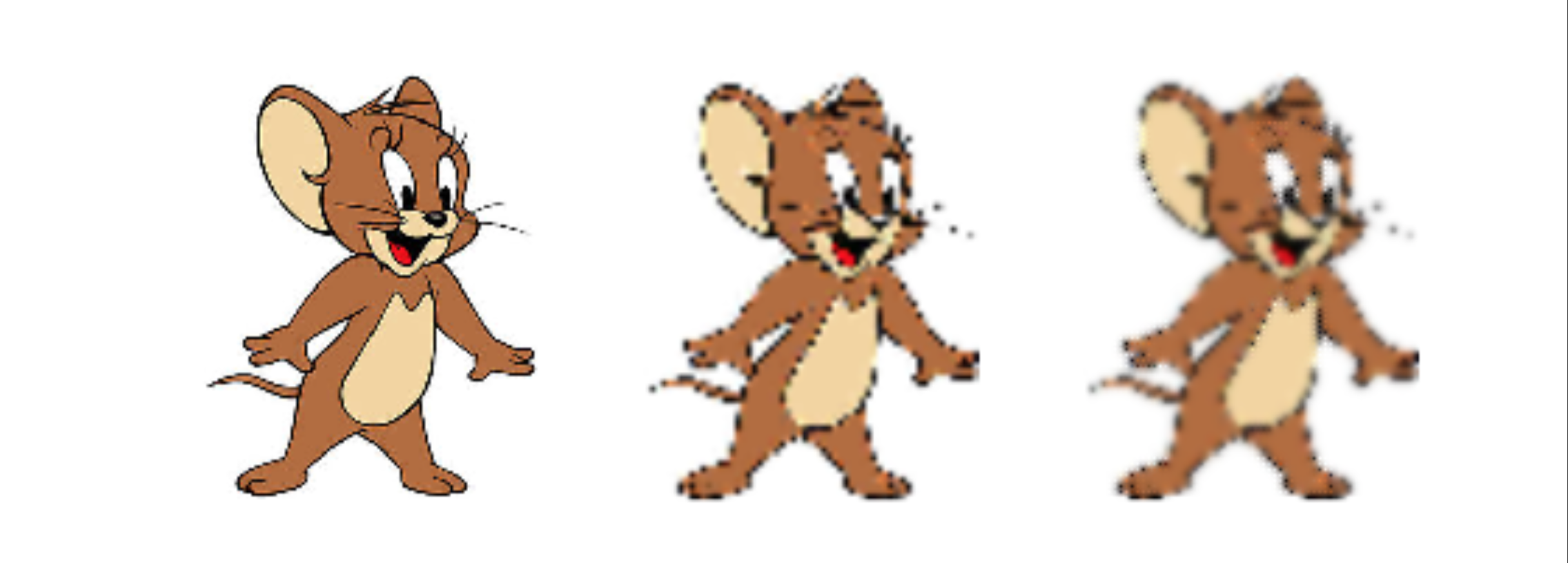
Figure 6: From L to R : Original Image. This image was downsampled by 4 to serve as input for the two
algorithms. Magnified image using bi-linear interpolation, magnified image using PDE regularisation
with t=3, 3x3 neighbourhood and 10 iterations.
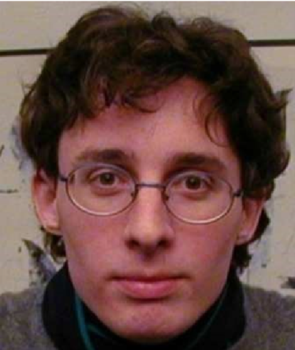
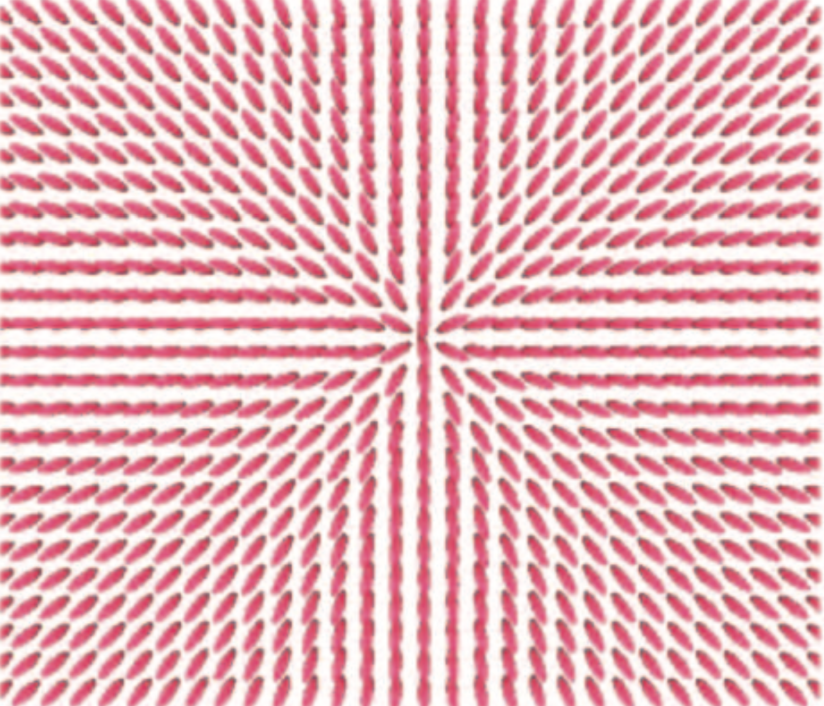
| Original Image | Flow | Flow Visualisation |
|---|---|---|
 |
 |
 |
 |
 |
 |
Figure 7: Input images, flow vectors and output images, with dt = 0.01, 100 iterations and sobel
gradient vectors for Hessian Matrix. Paralallised code, runs much faster compared to others.
Figure 8: From L to R : Input Image, image with 50 % pixels removed in 2x2 granularity, output
image with SSIM of 0.995, better than results with median filter. Also, median filter will
become less accurate on increasing the box sizes.
| Image with pixels missing | Restored Image |
|---|---|
 |
 |
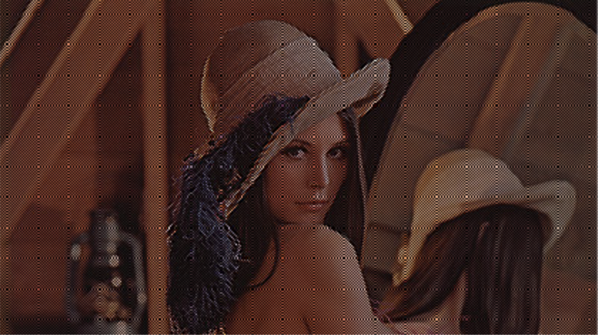
Figure 9: from L to R : image with 50 % pixels removed and SSIM = 0.23, restored image with t=4,
10 iterations with 3x3 neighbourhood, SSIM = 0.966 with original image.
- Saiteja Talluri - saiteja-talluri
- Shreyas Pimpalgaonkar - shreyas-7
- Meet Kathiriya
This project is licensed under the MIT License - see the LICENSE file for details.
