We implemented a Monte Carlo Tree Search (MCTS) from scratch and we successfully applied it to Tic-Tac-Toe game.
We performed tests using different allocated time to build MCTS (thinking time). We also could test several symmetrical and asymmetrical reward designs.
Summary of steps of MCTS model:
- At each turn do:
- during a time T, repeat the following steps:
- create a Tree (root) where each node is associated to a state of game
- select a leaf by UCB exploration
- create a child node from this leaf
- evaluate new state by roll out simulations
- backpropagate from leaf to the root by updating visit count and reward at each node of the path
- during a time T, repeat the following steps:
In our MCTS we used the following features:
- we used the following UCB for trees (UCT) formula with c = 1.4 :
- roll out simulations we performed by using random uniform policy
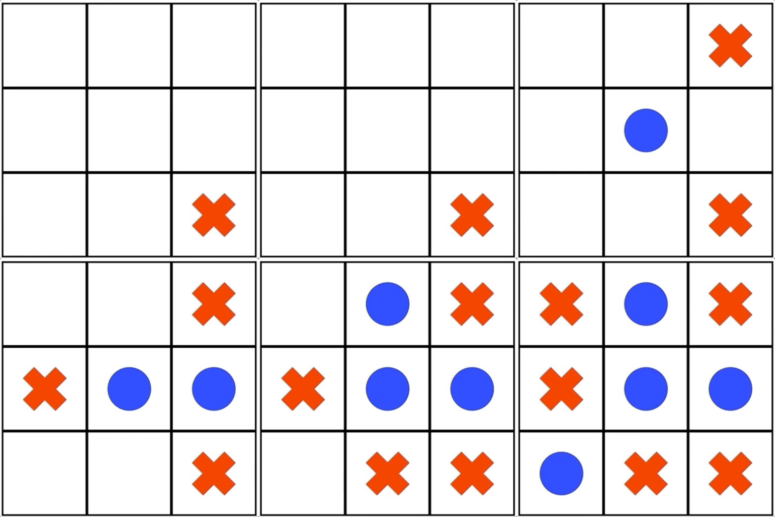
Here is a demo with 2 machines using MCTS playing against each other. Allocated thinking time is 0.1s. Reward designs are symmetrical with reward(win)=3 and reward(draw)=1.
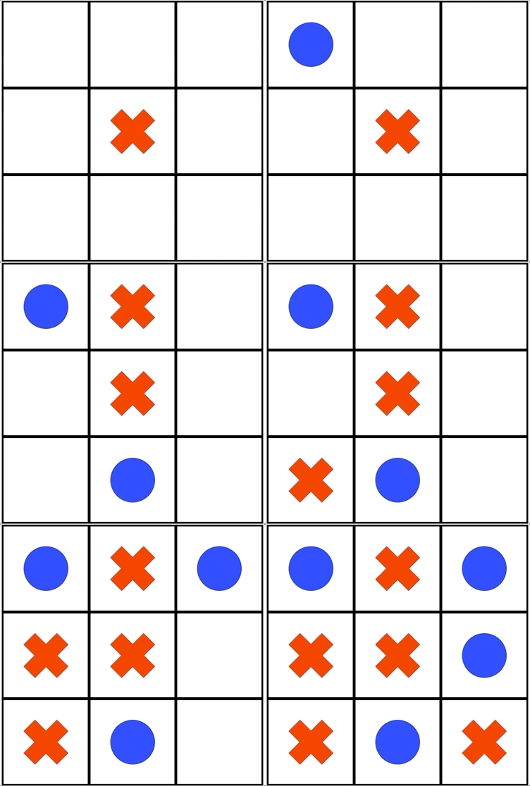
Here is a demo with 2 machines using MCTS playing against each other. Allocated thinking time is 0.3s. Reward designs are symmetrical with reward(win)=3 and reward(draw)=1.
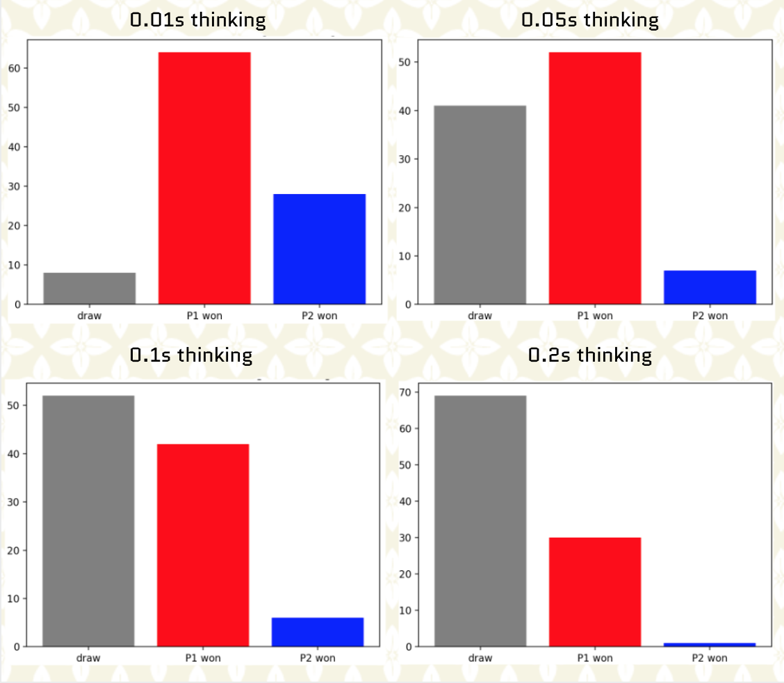
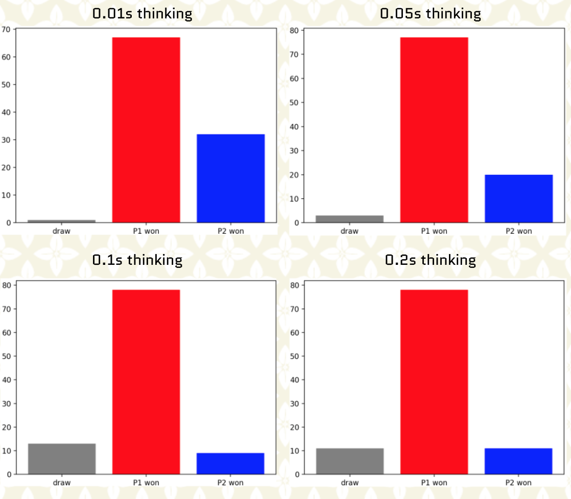
In the next figure we show the distribution of outcomes after we performed 100 games where we vary the allocated thinking time from 0.01s to 0.2s. Reward designs are symmetrical with reward(win)=3 and reward(draw)=1. Player 1 is the player to play first while player 2 is the player to play second.
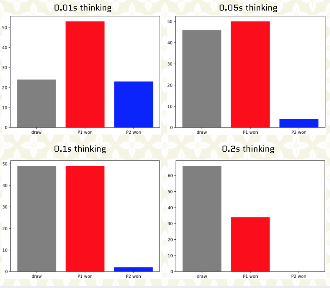
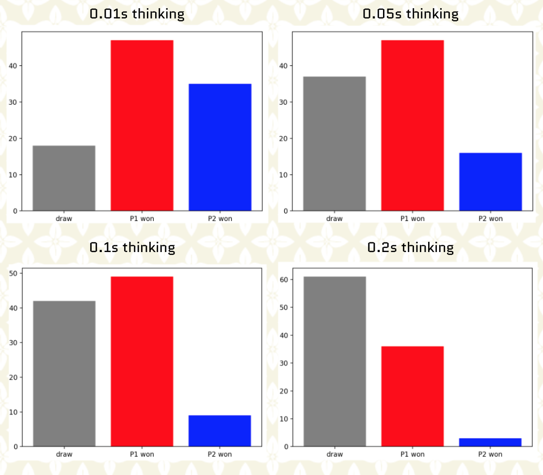
In the next figure we show the distribution of outcomes after we performed 100 games where we vary the allocated thinking time from 0.01s to 0.2s. Reward designs are asymmetrical with reward_1(win)=3 and reward_1(draw)=1 for player 1 (player to play first) and reward_2(win)=1 and reward_2(draw)=1 for player 2 (player to play second).
In the next figure we show the distribution of outcomes after we performed 100 games where we vary the allocated thinking time from 0.01s to 0.2s. Reward designs are symmetrical with reward(win)=1 and reward(draw)=0. Player 1 is the player to play first while player 2 is the player to play second.
In the next figure we show the distribution of outcomes after we performed 100 games where we vary the allocated thinking time from 0.01s to 0.2s. Reward designs are asymmetrical with reward_1(win)=1 and reward_1(draw)=0 for player 1 (player to play first) and reward_2(win)=1 and reward_2(draw)=1 for player 2 (player to play second).
From the previous plots we can make two observations:
-
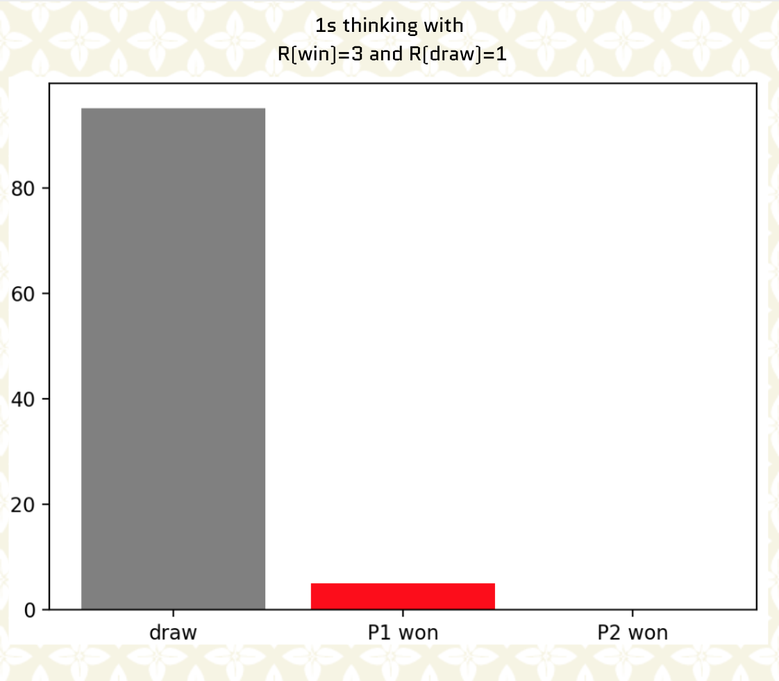
The more thinking time the higher chance the game outcome will be a draw.
-
The more thinking time the lower chance for player 2 to win.
-
Reward designs performance depend on thinking time.
-
Aggressive play is not optimal for player 1 nor for player 2.
-
Playing too safe (looking equally for draw or win) is not optimal for player 2, it is more effective to look more for victory, confirming the popular adage "attack is the better defense".
-
Reward design with reward(win)=3 and reward(draw)=1 seems to produce solid play for both player 1 and player 2

