ExaGAN
Basic GAN template for the Exalearn project: code for training a DCGAN on slices of N-body dark matter simulations and performing simple analysis tasks.
Datasets & Training
Tested setup
The code has been developed and run with the following software:
- numpy, scipy, matplotlib, h5py
- tensorflow 1.13.1
- tensorboard 1.13.1
- keras 2.2.4*
*Due to a bug in keras BatchNorm that is fixed on the master branch but not in v2.2.4, installing keras via pip or conda will lead to an error when using batch normalization along with the NCHW data format. To fix this, keras can be installed directly from the master branch, or these changes can be added to the keras installation.
Data fetching & pre-processing
The CosmoFlow N-body simulations dataset has a very large amount of data available, stored in HDF5 files. A small subset for testing can be downloaded from the cosmoUniverse_2019_05_4parE/22309462 directory. The following commands will fetch this data and take ~20k slices of size 128x128 from the simulations to be used as training data:
cd data
wget --recursive https://portal.nersc.gov/project/m3363/cosmoUniverse_2019_05_4parE/22309462
python slice_universes.py
The network performs better when there is a larger amount of data (e.g., 200,000 samples as in the original CosmoGAN paper).
Any given pixel in the simulation data has some value in [0, 4000] (there is technically no upper limit, but the max across all the simulations is roughly 4000), so the data must be transformed to the interval [-1,1] for more stable training. This normalization could be done in one of many possible ways (e.g. log transform, linear scaling, etc), but recent work has found the following transformation s(x) to be effective in capturing the high dynamic range of the simulations when mapping to [-1,1]:
s(x) = 2*x/(x+a) - 1
This is the normalization used in the current version of the code, with the parameter a=4.
Training
Training is done from the train.py script, which takes as arguments the configuration tag and run ID for the training run, e.g.:
python train.py base 0
This will set up a subdirectory base/run0/ in the expts subdirectory (the user must create expts before running this command), which will contain all the logs and checkpoints for the training run. The configuration tag base corresponds to a user-defined configuration (hyperparameters, architecture, etc) specified in config.yaml.
Training can be monitored using tensorboard. The model saves tensorboard checkpoints at user-defined intervals during training, and each checkpoint saves the discriminator and generator losses, some summary statistics, some generated samples, and plots for statistical analysis of the generated samples against the validation data.
Analysis
There are two main summary statistics which are useful metrics of the quality of generated samples -- the pixel intensity histogram and the power spectrum. The methods to compute and plot these metrics can be found in the utils/plots.py file.
The pixel intensity histogram compares the binned intensity per pixel in the generated samples against the validation set, and is essentially a measure of the "mass distribution" of the samples.
The power spectrum is a bit more challenging for the GAN to reproduce, as it is a "higher-order" statistic. The spectrum is calculated according to this method. A major caveat is that this method assumes 2D periodicity of the data, which is not true for slices of any size less than the full 512x512 sheet of the simulation domain (the simulations in the CosmoFlow dataset are cubes of size 512x512x512, with periodic boundary conditions). Thus, power spectra for small slices (e.g. 128x128) will look rather strange.
A template analysis script is provided in analyze_output.py, which loads pre-trained weights and generates samples to be displayed and analyzed statistically. Sample output of the script is shown below:
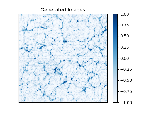
![]()
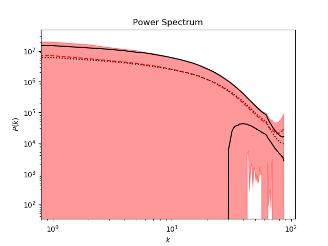
This particular result is from a model that was trained on a dataset of ~200k images and used the multi-channel rescaling method described in the section below.
Model description & details
Overview
The basic model is a simple DCGAN, essentially identical to that of the original CosmoGAN paper. Early tests showed the GAN having trouble capturing the tail of the distribution of pixel intensities (i.e., the pixels with very large values), which is heavily squashed by the transformation s(x) used to normalize the data. To ensure accuracy and useful gradients at both regimes of the data domain (pixels with lower values, which constitute the majority of the structures in filaments and voids, as well as the outlier pixels with very large values), we have developed a technique to augment the DCGAN model which we call multi-channel-rescaling (hereafter MCR).
This MCR technique simply concatenates a second image channel to the generator output, where the second channel is a different normalization of the data in the generated sample. The discriminator is then trained with the 2-channel images (the same transformation is applied to the training data). The normalization for the second channel which seemed to work best was simply a linear scaling of the data, scaled down by some large number (e.g., 1000), fed through a tanh to improve numerical stability. This method improved the quality and statistical validity of the output samples, although for larger images (e.g., of size 256x256) it is untested and may not be necessary.
Minor Details
A few modifications to the default Keras behavior were needed in parts of the code. These are minor modifications, and would likely not be necessary if this setup is ported to a different framework.
First, the default keras crossentropy loss assumes the network outputs probabilities (e.g., output of a sigmoid neuron), so it transforms back to logits and calls K.clip_by_value to ensure numerical stability -- however, we found this to be both unnecessary and actually destabilized training in many cases. The solution is simply to remove the sigmoid activation on the last layer of the discriminator and just compute the crossentropy loss directly from the logits using a custom keras loss function.
Second, the transposed convolution layers in keras (keras.layers.Conv2DTranspose) do not know their output shape before the model is compiled, so we have implemented a custom transposed convolution layer where the output shape is hardcoded to be computed according to the padding='same' configuration. Using this custom transposed convolution layer is required in order for keras to build the correct graph for the generator when the MCR technique is being used.
Authors
- Peter Harrington, Computational Research Division, LBNL -- pharrington@lbl.gov
Legal Information/License
ExaGAN Copyright (c) 2019, The Regents of the University of California, through Lawrence Berkeley National Laboratory (subject to receipt of any required approvals from the U.S. Dept. of Energy). All rights reserved.
If you have questions about your rights to use or distribute this software, please contact Berkeley Lab's Intellectual Property Office at IPO@lbl.gov.
NOTICE. This Software was developed under funding from the U.S. Department of Energy and the U.S. Government consequently retains certain rights. As such, the U.S. Government has been granted for itself and others acting on its behalf a paid-up, nonexclusive, irrevocable, worldwide license in the Software to reproduce, distribute copies to the public, prepare derivative works, and perform publicly and display publicly, and to permit other to do so.
For the license of this software, see LICENSE.md.