h3js

R bindings to H3, a hexagon-based geographic grid system via h3-js.

R bindings via native H3 C library can be found at h3r. h3r is much faster but requires installing h3 separately.

WARNING Only functions that take non-array input support vectorized operations currently. The return value of other functions when applying vectorized input may be unspecified. You should map over those input instead.

Installation

You can install the released version of h3js from CRAN with:

install.packages("h3js")

Development version can be installed with:

devtools::install_github("saurfang/h3js")

Core functions

library(h3js)
library(sf)
library(tidyverse)

# Convert a lat/lng point to a hexagon index at resolution 7
h3_index <- h3_geo_to_h3(37.3615593, -122.0553238, 7)
h3_index
#> [1] "87283472bffffff"

# Get the center of the hexagon
hex_center_coordinates <- h3_to_geo(h3_index)
hex_center_coordinates
#> [1]   37.35172 -122.05033

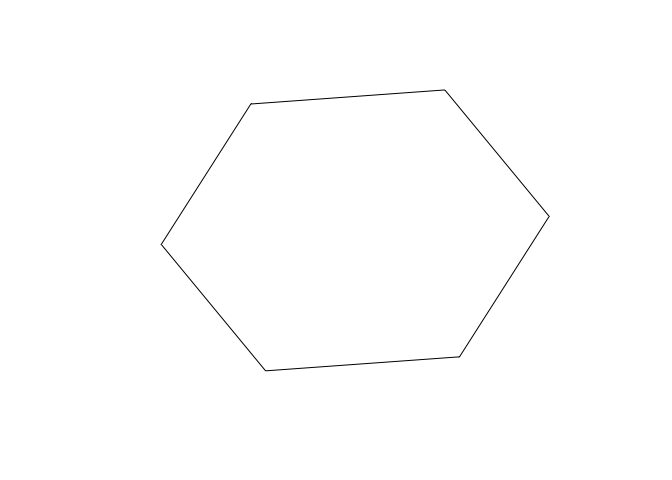
# Get the vertices of the hexagon
hex_boundary <- h3_to_geo_boundary(h3_index)
hex_boundary
#>          [,1]      [,2]
#> [1,] 37.34110 -122.0416
#> [2,] 37.35290 -122.0340
#> [3,] 37.36352 -122.0428
#> [4,] 37.36234 -122.0591
#> [5,] 37.35054 -122.0666
#> [6,] 37.33992 -122.0579

hex_boundary %>%
  # close polygon
  rbind(.[1,]) %>%
  # swap columns
  .[, c(2, 1)] %>%
  # convert to simple feature collection
  list() %>%
  st_polygon() %>%
  st_sfc() %>%
  plot()

Useful algorithms

# Get all neighbors within 1 step of the hexagon
h3_k_ring(h3_index, 1)
#> [1] "87283472bffffff" "87283472affffff" "87283470cffffff" "87283470dffffff"
#> [5] "872834776ffffff" "872834729ffffff" "872834728ffffff"

# Get the set of hexagons within a polygon
polygon <- list(
    c(37.813318999983238, -122.4089866999972145),
    c(37.7198061999978478, -122.3544736999993603),
    c(37.8151571999998453, -122.4798767000009008)
)
hexagons <- h3_polyfill(polygon, 7)
hexagons
#> [1] "872830828ffffff" "87283082effffff" "87283082affffff" "87283082bffffff"
#> [5] "872830876ffffff" "872830820ffffff" "872830870ffffff"

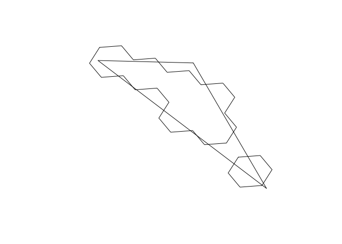
# Get the outline of a set of hexagons, as a GeoJSON-style MultiPolygon
coordinates <- h3_set_to_multi_polygon(hexagons, TRUE)

c(
  coordinates %>%
    map(~ matrix(.x, ncol = 2)) %>%
    map(list) %>%
    st_multipolygon() %>%
    st_sfc(),
  do.call(rbind, polygon) %>%
    # close polygon
    rbind(.[1,]) %>%
    # swap columns
    .[, c(2, 1)] %>%
    list %>%
    st_polygon() %>%
    st_sfc()
) %>%
  st_sf() %>%
  plot()

Benchmark

Houston <- list(lat = 29.7632836, lon = -95.3632715)

# single arguments
microbenchmark::microbenchmark(
  h3r::getIndexFromCoords(Houston$lat, Houston$lon, resolution = 5),
  h3_geo_to_h3(Houston$lat, Houston$lon, res = 5),
  h3r::getBoundingHexFromCoords(Houston$lat, Houston$lon, resolution = 5),
  h3_to_geo_boundary(h3_geo_to_h3(Houston$lat, Houston$lon, res = 5))
)
#> Unit: microseconds
#>                                                                     expr
#>        h3r::getIndexFromCoords(Houston$lat, Houston$lon, resolution = 5)
#>                          h3_geo_to_h3(Houston$lat, Houston$lon, res = 5)
#>  h3r::getBoundingHexFromCoords(Houston$lat, Houston$lon, resolution = 5)
#>      h3_to_geo_boundary(h3_geo_to_h3(Houston$lat, Houston$lon, res = 5))
#>       min        lq       mean    median        uq       max neval
#>    11.572   24.7375   41.46644   39.6285   52.1510   122.485   100
#>   742.427 1147.9030 1995.58544 1601.6880 2330.8450 11489.859   100
#>    17.031   27.6205  221.48883   50.7200   70.5675 16793.250   100
#>  1500.967 2104.0835 3411.27699 2920.7360 3930.8230 14837.502   100

# vectorized input
coordinates <- list(lat = runif(100, -90, 90), lon = runif(100, -180, 180))

microbenchmark::microbenchmark(
  pmap(coordinates, ~h3r::getIndexFromCoords(.x, .y, resolution = 5)),
  h3_geo_to_h3(coordinates$lat, coordinates$lon, res = 5)
)
#> Unit: microseconds
#>                                                                 expr
#>  pmap(coordinates, ~h3r::getIndexFromCoords(.x, .y, resolution = 5))
#>              h3_geo_to_h3(coordinates$lat, coordinates$lon, res = 5)
#>       min       lq     mean   median       uq       max neval
#>  1508.317 1847.437 3011.063 2236.570 2907.621 38565.621   100
#>   817.205 1114.620 1768.592 1368.635 1822.631  8248.186   100