Trajectory-Estimation-Of-A-Projectile

Objective: To fit the best curve for the ball’s trajectory using the input from two different videos and compare different fitting methods on basis of efficiency, time of execution and goodness of fit etc. For detailed report checkout this link.

Input videos

sls.py

a) This file has the standard least square function and it uses numpy for matrix operations. To implement this function X and Y matrices are created using the data points found from the video.

b) As the curve is a parabola the equation to fit the points will be y = a x 2 + b x + c . Assuming n data points, the X matrix will be an n3 matrix, having x 2 , x and 1 values in the columns and matrix Y will be an n1 matrix with y values.

c) To find the least squares solution, we need to minimize the error equation by equating its derivative to zero. So, we will end up the following equation:

(X.T)XB = (X.T)Y

B = (X.TX)(X.TY)

tls.py

a) This file has the total least square function and it uses numpy and custom built svd function to calculate the tls solution. To implement this function X and Y matrices are created using the data points found from the video.

b) To fit the points using total least squares we will use c y = a x 2 + b x + d . Also, assuming the data is passing through origin we will drop the constantvalue i.e the equation will be c y = a x 2 + b x. Assuming n data points, the X matrix will be an n2 matrix having x 2 and x values in the columns and matrix Y will be an n1 matrix with y values.

c) To find the solution we have to minimize the total least square error i.e we will equate its derivative to zero and will find the final equation.

d) Now to construct the final matrix we will combine X and Y matrices and assign them to Z, further we will find the Singular Value Decomposition(SVD) of the Z matrix, which will give the decomposition of combined matrix as:

Z=UΣV.T

e) Transpose the V.T matrix to get the coefficients matrix V. Now, separate the initial(a,b) and the last coefficient(c) from V. Finally, divide the initial coefficients by c to get the final coefficients. Return them to the main.py file.

ransac.py

a) This file has the implementation of the RANSAC function and it uses numpy, math, random, scipy libraries along with sls.py file.

b) For N iterations :-

● Select randomly a subset of s data points from the list of all data points.

● Fit a model to those data points using std_least_square function(it will fit perfectly, because we have 3 points).

● After fitting the model, solve the constraint optimization problem using scipy for each point and find the distance from the point to the curve.

● After finding the distance compare it with the threshold(t), if the distance is less than t increment the inlier_count. Do this for all points for a single model.

● Now, if the new model has the higher inlier_count update the best_model and max_inlier_count variables with result and inlier_count respectively. ○ best_model ← result

repeat.....

Output

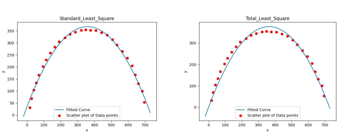
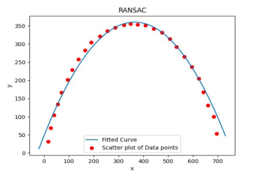
Video without Noise

For this video,standard least squares technique gives the least error(4500.34), and takes the least time to execute(0.0008s), whereas total least squares takes more time(0.0019) and has a significant error(9128.40). Also, as the RANSAC is a probabilistic model, its performance depends upon the number of iterations(i.e parameters), so it gives varying results, also it takes a significant amount of time to fit due to its high time complexity(~O( n 3 )). So, for the first video standard least squares solution should be opted.

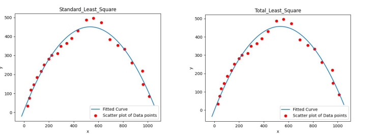
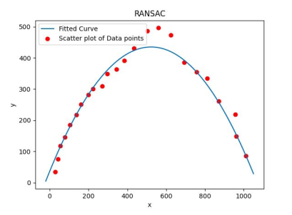
Video with Noise

The second video contains a lot of noise, thus it has many outliers present. Now, standard least squares and total least squares methods don’t take outliers into consideration and thus try to fit them into the curve, but the ransac method takes them into consideration and rejects the outliers, to fit a better curve. Here, although the RANSAC method takes some time to compute due to its high time complexity, but it has the least error(7430.49), which makes it desirable for these cases. (NOTE: The error is calculated after removing the outliers.) So, for the second video RANSAC algorithm should be opted.

How to run the code

Change the directory of input video file in the main1.py file
```
  video = "Ball_travel_10fps.mp4"
```
Run the main.py file.

savnani5/Trajectory-Estimation-Of-A-Projectile