jsd-mlflow-examples

This is a collection of MLflow project examples that you can directly run with mlflow CLI commands or directly using Python.

The goal is provide you with additional set of samples, focusing on machine learning and deep learning examples, to get you quickly started on MLFlow. In particular, I focus on Keras and borrow and extend examples from Francois Cholllet's book: Deep Learning with Python

1. Keras MLP Binary Classification Model.

This is a simple Keras neural network model with three layers, one input, one hidden, and one output layer. It's a simple linear model: y=Mx. Given a random numbers of X values, it learns to predict it's Y value, from a training set.

This Multi-layer Perceptron (MLP) for binary classification model's sources have been modified from this gist. You can use other network models from this gist in a similar fashion to experiment.

The arguments to run this simple MLP Keras network model are as follows:

--drop_rate: Optional argument with a default value is 0.5.
--input_dim : Input dimension. Default is 20.
--bs: dimension and size of the data. Default is (1000, 20)
--output: Output to connected hidden layers. Default is 64.
--train_batch_size: Training batch size. Default is 128
--epochs: Number of epochs for training. Default is 20.

To experiment different runs to evaluate metrics, you can alter the arguments, for example, expand the size of network by providing more output to the hidden layers. Or you may change the drop_rate or train_batch_size — all will alter the loss and accuracy of the network model.

To run the current program with just python and yet log all metrics, use the following command:

python keras/keras_nn_model.py

python keras/keras_nn_model.py --output=128 --epochs=10

python keras/keras_dnn/main_nn.py --output=128 --epochs=10

It will log metrics and parameters in the mlruns directory.

Alternatively, you can run using the mlflow command.

mflow run . e -keras-nn-model

mlflow run . -e keras-nn-model -P drop_rate=0.3 -P output=128

The next two examples are from Deep Learning with Python. While the Jupyter notebooks can be found here, I have modified the code to tailor for use with MLflow. The description and experimentation remain the same, hence it fits well with using MLflow to experiment various capacity of networks layers and suggested parameters to evaluate the model.

2. Classifying Movie Reviews: a Keras binary classification example.

This part comprises of code samples found in Chapter 3, Section 5 of Deep Learning with Python. The borrowed code from the book has been modularized and adjusted to work with MLflow, and it fits well since Francois suggests some experimentation parameters to tweak to see how the model metrics change.

Two-class classification, or binary classification, may be the most widely applied kind of machine learning problem. In this example, we will learn to classify movie reviews into "positive" reviews and "negative" reviews, just based on the text content of the reviews.

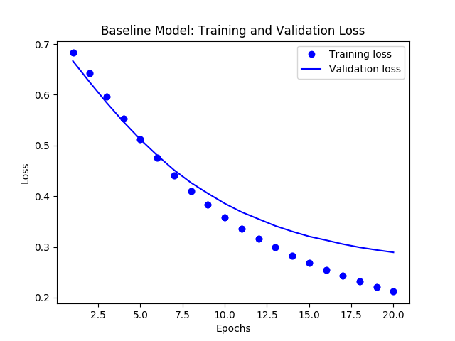
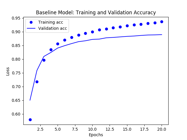
This example creates two types of models for you to work with. First, it creates a baseline model with default parameters:

loss function as rmstrop
binary_crossentropy for metrics
learning rate as 0.001
a Keras neural network model with
- An input layer with input_shape (10000, )
- 1 hidden layer with output = 32
- 1 Output layer with output = 1
- All layers use relu as an activation function except for sigmod that is used in the final output layer.
epochs = 20; batch_size=512

And the second model can me created for experimenting by changing any of the these parameters to measure the metrics:

Use 2 or more hidden layers
Use 4, 8, 12 or 16 epochs
Try hidden layers with output 32, 64 or 128 and see if that affects the metrics
Try to use the mse loss function instead of binary_crossentropy.

In both cases, the model will create images for training and validation loss/accuracy images in the images directory

How to Use MLflow to Experiment, Log Metrics and Artifacts

To run the current program with just python and default or supplied parameter and yet log all metrics, use the following command:

cd imdbclassifier

python main_nn.py

Note: You will need to do pip install imdbclassifier

To experiment different runs, with different parameters suggested above, and evaluate new metrics, you can alter the arguments. For example, expand the size of network by providing more output to the hidden layers. Or you may change the hidden_layers or epochs or loss function — all will alter the loss and accuracy of the network model. For example,

python main_nn.py  # hidden_layers=1, epochs=20 output=16 loss=binary_crossentropy
python main_nn.py --hidden_layers=3 --output=16 --epochs=30 --loss=binary_crossentropy 
python main_nn.py --hidden_layers=3 --output=32 --epochs=30 --loss=mse

It will log metrics and parameters in the mlruns directory.

Alternatively, you can run using the mlflow command.

Note: mlflow run.. may take longer as it needs to create and setup an environment by and download and installing dependency packages listed in conda.yml

mlflow run keras/imdbclassifier -e main

mlflow run keras/imdbclassifier -e main -P hidden_layers=3 -P output=32 -P epochs=30 -P loss=mse

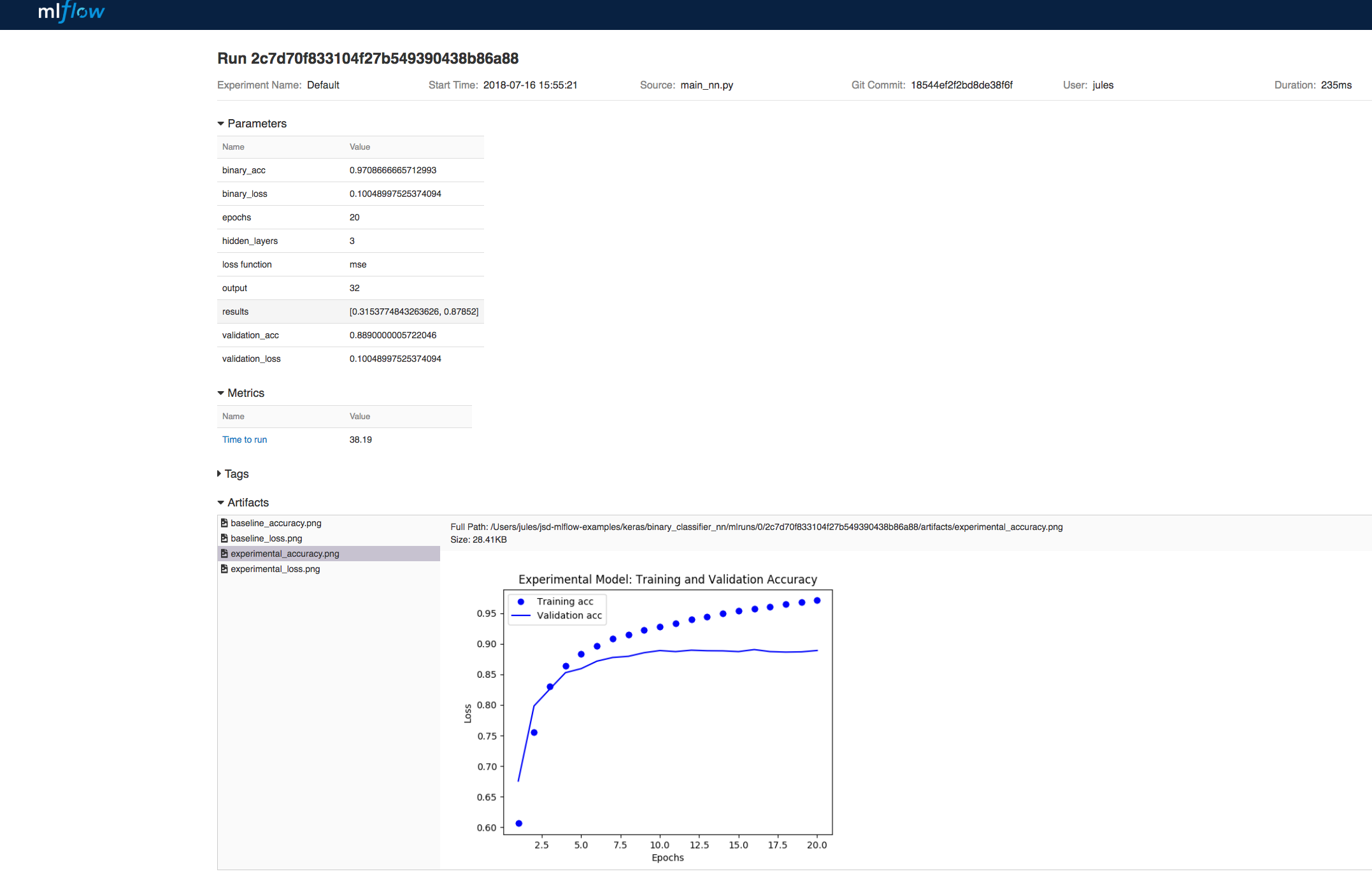
To view the output of either runs, launch the mlflow ui:

mlflow ui

These runs will not only log metrics for loss and accuracy but also log graphs generated from matplotlib for perusal as part of visual artifacts.

Finally, you can run this in a Jupyter Notebook:

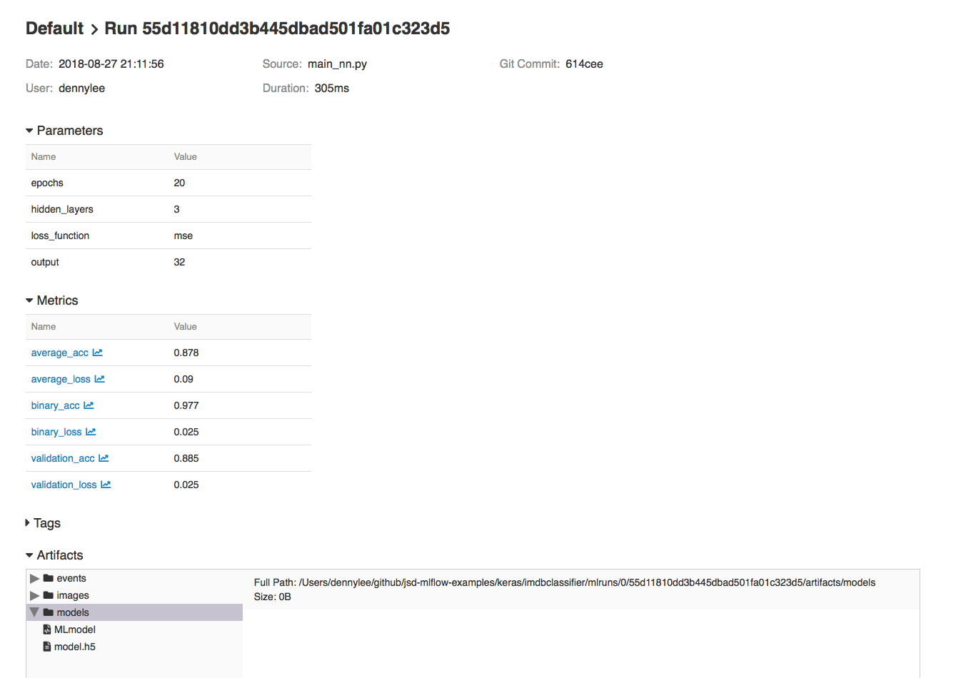
How to Use MLflow to Load Saved Model

When executing your test runs, the models used for these runs are also saved via the mlflow.keras.log_model(model, "models") within train_nn.py. Once you have found a model that you like, you can re-use your model using MLflow as well. Your Keras model is saved in HDF5 file format as noted in MLflow > Models > Keras.

This model can be loaded back as a Python Function as noted noted in mlflow.keras using mlflow.keras.load_model(path, run_id=None).

To execute this, you load the model you had saved within MLflow by going to the MLflow UI, selecting your run, and copying the path of the stored model as noted in the screenshot below.

Using the code sample reload_nn.py, you can load your saved model and re-run it using the command:

python reload_nn.py --hidden_layers=3 --output=32 --load_model_path='/Users/dennylee/github/jsd-mlflow-examples/keras/imdbclassifier/mlruns/0/55d11810dd3b445dbad501fa01c323d5/artifacts/models'

mlflow run keras/imdbclassifier -e reload -P output=4 -P load_model_path=/Users/jules/jsd-mlflow-examples/keras/imdbclassifier/keras_models/178f1d25c4614b34a50fbf025ad6f18a

How to Reproduce a Run or an Experiment

As part of machine development life cycle, reproducibility of any experiment by team members or ML developers is imperative. Often you will want to either retrain or reproduce a run from several past experiments to reproduce the results for sanity or audibility.

One way is to manually read the parameter from the MLflow UI for a particular run_uuid and rerun using main_nn.py or reload_rn.py, with the original parameters arguments.

Another preferred way is to simply use run_uuid, and use it with reproduce_nn.py. This command will fetch all the right hyper-parameters used for training the model and will recreate or reproduce the experiment, including building, training, and evaluating the model. To see the code how the new Python tracking and experimental APIs are used, read the source reproduce_nn.py.

You can run these either of two ways:

python reproduce_run_nn.py --run_uuid=7261d8f5ae5045d4ba16f9de58bcda2a
python reproduce_run_nn.py --run_uuid=7261d8f5ae5045d4ba16f9de58bcda2a [--tracking_server=URI]

mlflow run keras/imdbclassifier -e reproduce -P run_uuid=7261d8f5ae5045d4ba16f9de58bcda2a
mlflow run keras/imdbclassifier -e reproduce -P run_uuid=7261d8f5ae5045d4ba16f9de58bcda2a [--tracking_server=URI]

The output from the above runs. By default the tracking_server defaults to the local 'mlruns' directory. ...

The output from the above runs. By default the tracking_server defaults to the local 'mlruns' directory.

...
Using TensorFlow backend.
run_uuid: 5374ba7655ad44e1bc50729862b25419
hidden_layers: 4
output: 4
epochs: 25
loss: mse
load model path: /tmp
tracking server: None
2018-09-12 10:25:24.378576: I tensorflow/core/platform/cpu_feature_guard.cc:141] Your CPU supports instructions that this TensorFlow binary was not compiled to use: SSE4.1 SSE4.2 AVX AVX2 FMA
Experiment Model:
Writing TensorFlow events locally to /var/folders/b7/01tptb954h5_x87n054hg8hw0000gn/T/tmpiva13sry

Train on 15000 samples, validate on 10000 samples
Epoch 1/25
15000/15000 [==============================] - 3s 189us/step - loss: 0.2497 - binary_accuracy: 0.5070 - val_loss: 0.2491 - val_binary_accuracy: 0.4947
...

How to run the model

Now that you have a model, you can type in your own review by loading your model and executing it. To do this, use the predict_nn.py against your model:

python predict_nn.py --load_model_path='/Users/dennylee/github/jsd-mlflow-examples/keras/imdbclassifier/mlruns/0/55d11810dd3b445dbad501fa01c323d5/artifacts/models' --my_review='this is a wonderful film with a great acting, beautiful cinematography, and amazing direction'

mlflow run keras/imdbclassifier -e predict -P load_model_path='/Users/jules/jsd-mlflow-examples/keras/imdbclassifier/keras_models/178f1d25c4614b34a50fbf025ad6f18a' -P my_review='this is a wonderful film with a great acting, beautiful cinematography, and amazing direction'

The output for this command should be something like:

Using TensorFlow backend.
load model path: /tmp/models
my review: this is a wonderful film with a great acting, beautiful cinematography, and amazing direction
verbose:  False
Loading Model...
Predictions Results:
[[ 0.69213998]]

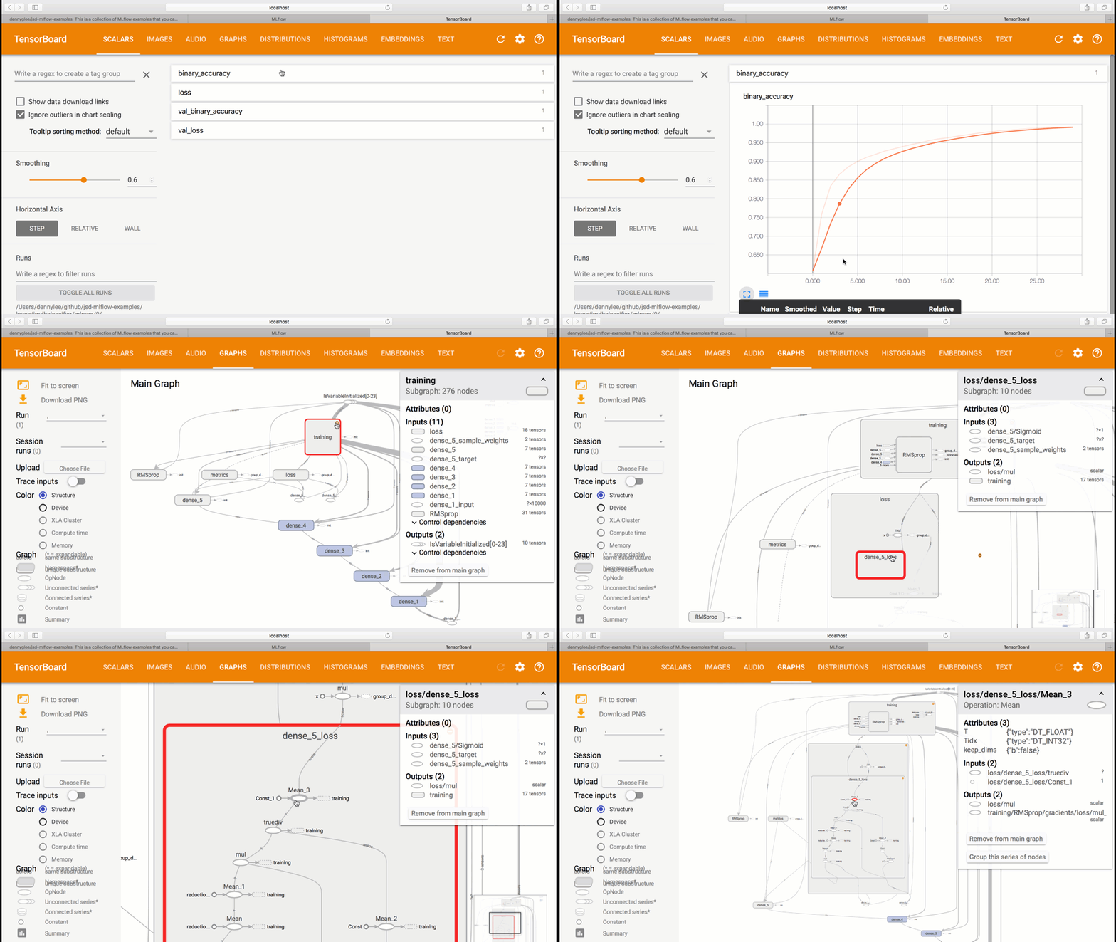
How Visualize TensorFlow Graphs with TensorBoard

If you have TensorBoard installed, you can also visualize the TensorFlow session graph created by the train_models() within the train_nn.py. For example, after executing the statement python main_nn.py, you will see something similar to the following output:

Average Probability Results:
[0.30386349968910215, 0.88336000000000003]

Predictions Results:
[[ 0.35428655]
 [ 0.99231517]
 [ 0.86375767]
 ..., 
 [ 0.15689197]
 [ 0.24901576]
 [ 0.4418138 ]]
Writing TensorFlow events locally to /var/folders/0q/c_zjyddd4hn5j9jkv0jsjvl00000gp/T/tmp7af2qzw4

Uploading TensorFlow events as a run artifact.
loss function use binary_crossentropy
This model took 51.23427104949951  seconds to train and test.

You can extract the TensorBoard log directory with the line stating Writing TensorFlow events locally to .... That is, to run Tensorboard, you can run the following command:

tensorboard --logdir=/var/folders/0q/c_zjyddd4hn5j9jkv0jsjvl00000gp/T/tmp7af2qzw4

Click on graph and you can visualize and interact with your session graph.

3. Classifying Newswires: a multi-class Keras classification example

This contains the code samples found in Chapter 3, Section 5 of Deep Learning with Python.

In the above model we saw how to classify vector inputs into two mutually exclusive classes using a densely-connected neural network. But what happens when you have more than two classes?

In this section, we will build a network to classify Reuters newswires into 46 different mutually-exclusive topics. Since we have many classes, this problem is an instance of "multi-class classification", and since each data point should be classified into only one category, the problem is more specifically an instance of "single-label, multi-class classification". If each data point could have belonged to multiple categories (in our case, topics) then we would be facing a "multi-label, multi-class classification" problem.

schipiga/jsd-mlflow-examples