| Author: | Ralf Schlatterbeck <rsc@runtux.com> |
|---|
This is an attempt to rewrite the original MININEC3 basic sources in Python. Standard use-case like computation of feed impedance and far field are implemented and are quite well tested. There is only a command line interface.
An example of using the command-line interface uses the following
12-element Yagi/Uda antenna originally presented by Cebik [6] without
the resistive element loading and with slight corrections to the element
lengths to make the antenna symmetric (the errors in the display in
Cebik's article may be due to a display issue of the program used that
displays negative numbers with less accuracy than positive numbers).
You can get further help by calling pymininec with the --help
option. The command-line options for the 12-element antenna example
(also available in the file test/12-el.pym) are:
pymininec -f 148 \
-w 22,-.51943,0.00000,0,.51943,0.00000,0,.00238 \
-w 22,-.50165,0.22331,0,.50165,0.22331,0,.00238 \
-w 22,-.46991,0.34215,0,.46991,0.34215,0,.00238 \
-w 22,-.46136,0.64461,0,.46136,0.64461,0,.00238 \
-w 22,-.46224,1.03434,0,.46224,1.03434,0,.00238 \
-w 22,-.45989,1.55909,0,.45989,1.55909,0,.00238 \
-w 22,-.44704,2.19682,0,.44704,2.19682,0,.00238 \
-w 22,-.43561,2.94640,0,.43561,2.94640,0,.00238 \
-w 22,-.42672,3.72364,0,.42672,3.72364,0,.00238 \
-w 22,-.41783,4.53136,0,.41783,4.53136,0,.00238 \
-w 22,-.40894,5.33400,0,.40894,5.33400,0,.00238 \
-w 22,-.39624,6.0452,0,.39624,6.0452,0,.00238 \
--theta=0,5,37 --phi=0,5,73 \
--excitation-pulse=33 > 12-el.pout
When the command line options are in a file, comments (using '#' at the start of the line) can be added. Users on Linux can run this using (I'm sure Windows users can come up with a similar command-line on Windows):
pymininec $(sed '/^#/d' test/12-el.pym) > 12-el.pout
or using grep:
pymininec $(grep -v '#' test/12-el.pym) > 12-el.pout
This removes comments from the .pym file and passes the result as
command-line parameters to pymininec.
The resulting output file contains currents, impedance at the feedpoint
and antenna far field in dBi as tables. The output tries to reproduce
the format of the original Basic implementation of Mininec.
There is a -h or equivalent --help option that gives a brief
summary of the available options. All long options can be abbreviated to
their shortest unique prefix. Values often follow an option, either as a
separate argument (with a space between option and value) or directly
connected to the option with =, see the example in the introduction.
The typical usage defines the frequency using the -f or
--frequency option, frequency is specified in MHz. In addition it
often makes sense to define a frequency sweep: The start frequency of
the sweep is the value given by the -f option, with the options
--frequency-increment=<increment> and --frequency-steps=<steps>
specifying how many steps with size increment are performed.
Next the geometry of the antenna is defined. In the current version there are only wires that can be specified. A wire definition takes the form:
--wire [tag,]<nseg>,<x1>,<y1>,<z1>,<x2>,<y2>,<z2>,<radius>
where (x1, y1, z1) specifies the first endpoint of the wire in
carthesian coordinates, (x2, y2, z2) defines the second endpoint of the
wire, and finally the radius is specified. All lengths and coordinates
are in meter, but see below for the --geo-scale option. The leading
tag is optional and is used to refer back to the wire with other
options, e.g. when specifying the feedpoint or loads on the antenna. If
no tag is specified, wires are numbered starting with the highest
specified tag number or if no tag is specified, one. It is recommended
to not mix wires with and without tag. The parameter nseg specifies
the number of segments the wire is split into for computation.
By default wires are segmented into equal-length segments. Segments should not be longer than 1/20 the shortest wavelength λ. Mininec typically produces results with a resonant frequency slightly too high (so the antenna is too long), this can be improved by using a high number of segments.
An alternative is to use segments that are not equal-length. This can be
done using the --taper-wire option. It gets 2–4 parameters. The first
is the wire tag to identify the wire that should be length-tapered. The
second parameter specifies from which end of the wire tapering should be
performed. The end can either be 1, 2 for first and second end,
respectively, and 3 for both ends. The third and fourth parameters
specify the minimum and maximum segments lengths, respectively. A
minimum segment length of 2.5 the radius is enforced: If segments get
shorter, the thin-wire asumption is violated and results will be wrong.
The tapering starts out with the shortest possible segment under the
constraints of minimum and maximum segment length and doubles the
segment length until the maximum is reached, it also stops making
segments longer when subsequent segments would have to be shorter than
the current segment to keep the number of segments.
Sometimes it is necessary to modify parts of the geometry. Three
geometry transformation options are available. To rotate part or all of
an antenna the --geo-rotate option is used. It gets 4–5 comma
separated parameters. The first is a numeric key for sorting geo
transformations: The order of transformations matters, so it is
necessary to specify the order. The next three options are the rotations
around X- Y- and Z-axis. An optional fifth parameter specifies the geo
object tag (e.g. wire tag) to rotate. If no tag is given the whole
antenna is rotated. If more than one rotation is non-zero, the X-axis
rotation is performed first, then the Y-axis rotation and finally the
Z-axis rotation.
The --geo-translate option again gets 4–5 comma separated
parameters. The first is again a sort key. The next three parameters
specify displacement in X- Y- and Z-direction. Finally again a tag can
be specified to define the geometry object to translate. If left out the
whole antenna is moved. This is often useful for modifying the height
above ground of an antenna: The whole antenna can be shifted up without
having to edit all the Z-components of all geometry elements.
Finally the --geo-scale option scales all geometry parameters
(including the radius) by a given factor. The factor is the first
parameter, an optional second parameter again gives a geometry tag. If
the tag is omitted the whole antenna is scaled. The scaling is always
applied last so that the --geo-translate option applies to the
original lengths.
An example is in test/vdipole-rot-trans.pym: This has the geo
transformation options:
--geo-rotate=1,0,0,90
--geo-rotate=2,90,0,0
--geo-translate=3,0,0,7.33
This first rotates the antenna around the Z-axis by 90° (sort-key 1),
then around the X-axis by 90° (sort-key 2), and finally the whole
antenna is shifted up by 7.33m (sort-key 3). Note that in this case we
cannot combine the rotation around Z- and X-axes into a single
--geo-rotate option because this would rotate first around the
X-axis which would get a different result than first rotating around the
Z-axis.
Mininec uses the concept of a pulse for defining where feed voltages
and loads apply. Think of a pulse as the point between two segments.
This means that at the end of wires (unless a second or third wire
connects there) there is no pulse. So a single wire consisting of 3
segments contains only 2 pulses, or generally a wire with N segments
contains N-1 pulses. Pulses are automatically numbered starting with 1.
When a new wire is defined joining the endpoint of an already-existing wire which has no connections yet, the pulse at the wire junction is "owned" by the new wire: It becomes the first pulse on the new wire.
If more than two wires join at a coordinate, it is not a good idea to allocate a feedpoint or load to that pulse: The feedpoint or load would be only between two of the three or more wires. In such a case it is better to insert a small length of wire where the feedpoint or load is placed as in the following picture.
For an antenna at least one feedpoint needs to be defined. This is done
using the --excitation-pulse option. The pulse number is either
absolute over all pulses of the antenna or a comma-separated sequence
of two values can be specified where the first is the pulse number
relative to the wire specified by the second number, the wire tag.
By default the excitation voltage is 1V but this can be changed by
specifying a --excitation-voltage option which gets a complex number
in volts. If multiple feedpoints are defined this is done by multiple
--excitation-pulse and --excitation-voltage options.
Adding loads to an antenna structure is a two-step process. In the first step the loads are defined. In the second step they are attached to pulses.
The easiest load type is specified with the -l or --load option.
It gets a complex number as argument. Note that this simple load type
does not change with frequency. Simple loads are sorted first when
attaching loads.
Laplace loads are the most general type of load. With it combinations of
lumped element loads can be modeled. In a combination of serial and
parallel lumped components, an inductance is modeled with L*s, a
capacitance is modeled with 1/(C*s) and a resistance with R. After
analyzing a complex circuit, a polynomial of s results in the numerator
and denominator of a fraction. The denominator is specified with the
--laplace-load-a option and the numerator with the
--laplace-load-b option. Both take a comma-separated list of real
numbers, representing the coefficients of the polynomial in increasing
order of exponentials. Laplace loads are sorted last when attaching
loads.
Another load type that is internally based on laplace loads is specified
with the --rlc-load option. It gets three parameters, the resistance
in Ohm, the inductance in Henry and the capacitance in Farad. A zero
in the Farad position indicates a short instead of a capacitance. All
three lumped components are connected in series. RLC loads are sorted
second when attaching loads.
Finally trap loads – which are also based on laplace loads internally
– allow the specification of traps in an antenna. They
consist of a serial connection of a resistor with an inductance
(modeling the non-zero resistance of a real inductance) in parallel with
a capacitance. The --trap-load option gets three comma-separated
real numbers, the resistance, the inductance, and the capacitance in
Ohm, Henry, and Farad, respectively. Trap loads are sorted third when
attaching loads.
Loads are attached to pulses with the --attach-load option. The
option takes 2–3 comma separated parameters. The first is the load
index. The load indeces are computed by iterating over all simple loads,
then all RLC loads, then all trap loads and finally all laplace loads
assigning them a load index starting with one.
Non-ideal wires have distributed conductivity. With the option
--skin-effect-conductivity distributed conductivity of a wire can be
specified. Alternatively the --skin-effect-resistivity option can be
used if the resistivity of the wire is known. Both option get one or two
parameters. The first parameter is the conductivity or resistivity,
respectively. The second optional parameter specifies the geometry
(e.g. wire) tag. If no tag is given, the skin effect load is attached to
all geometry objects.
Wires can have insulation. The effect of insulation on the distributed
impedance of a wire is modeled with the --insulation-load option. It
gets 2–3 parameters. The first parameter specifies the radius of the
wire including insulation. The second specifies the relative
permittivity of the insulation. The third optional parameter specifies
the geometry (e.g. wire) tag. If no tag is given the insulation load is
attached to all wires.
At most one insulation load and at most one skin effect load can be specified per wire.
Ground can be specified with the --medium option. If not given, free
space is asumed. Multiple --medium options can be specified in which
case the subsequent media are either concentric around the first ground
or linearly allocated in X-direction. The --boundary option
specifies if the media are concentric (--boundary=circular) or in
X-direction (--boundary=linear) the default is a linear boundary.
The --medium option gets 3–4 comma-separated parameters, the
permittivity (dielectric constant), the conductivity, and the height.
If the first three are zero, ideal ground is asumed. With ideal ground
only a single --medium option is allowed.
The fourth parameter gives the width of the ground (the distance to the
next medium), this is a length in X-direction for linear boundary and a
radius for circular boundary. The fourth parameter is not used for the
last --medium option.
Note that you typically want negative heights for media further out, this allows modelling of summits. Mininec allows the specification of higher grounds but the results will be questionable as no reflection at the higher ground is modelled. The first medium must always be at height zero.
For the first medium, radials can be specified. Radials are allowed only
for non-ideal ground. The option --radial-count gives the number of
radials. The option --radial-radius gives the radius of the
radial-wires. Specifying radials will automatically select circular
boundary. The length of the radials is defined by the distance to the
next medium. So with radials at least two --medium options are
required.
With the --option option it can be specified what outputs are
computed and printed. This option can be specified multiple times.
It can take the arguments far-field, far-field-absolute,
near-field, and none. When none is specified as the only
option, only currents and feed point impedance are printed.
The far-field options selects printing of the far field in dBi.
The far-field-absolute option selects printing of the far field in
V/m. This option can be modified by specifying a different power level
using the --ff-power` option and the --ff-distance option to
specify the distance in radial direction of the far field measurement
point. Far field measurements are taken at elevation and azimuth angles
specified with the --theta and --phi options, respectively.
The elevation angle theta is measured from the zenith while the azimuth
angle phi is measured from the X-axis. Both, the --theta and the
--phi option take tree comma-separated arguments: The start angle,
the angle increment, and the number of angles. By default, theta is
"0,10,10", so it runs from the zenith to ground in 10 degree steps. The
default for phi is "0,10,37", so it runs around the azimuth circle in 10
degree steps, computing the 0° and 360° on the X-axis value twice. This
is needed for some 3d-plotting tools for plotting a closed surface for
the 3d gain pattern.
The --option=near-field specifies printing of the near field.
This also needs specification of the --near-field option which gets
9 comma-separated parameters: The first three define the start (x, y, z)
coordinate of near-field measurements, the next three define the
increment of far field measurements and the last three define the number
of increments in each direction. With the --nf-power option it
is possible to modify the power level for the near field computation.
Without any --option, far field is printed if no near field
options are present.
With the option --output-cmdline the given command-line options can
be printed. This is useful for tests and when using the API: All options
can be written out to reproduce the current settings. The option takes a
file name as an argument.
With the option --output-basic-input, input for the original Mininec
code in Basic can be printed. The Basic code uses prompts to ask the
user for input. With this option the complete user input can be
generated. Running the Basic code with Yabasi, the user input can be
fed into the Basic program with the -i option which is useful for
comparing the values computed by pymininec to the values computed by the
original Basic code. The option takes a file name as an argument.
With the -T or --timing option, printing of runtimes of various
parts of the computation is requested. The option takes no arguments.
Starting with version 1 there is a command-line option -T which
outputs computation timings on the standard error output. This was used
for measuring the results of recent vectorization of computations.
Speedups are roughly:
- About a factor of 50 for computation of the impedance matrix. So we're down from around 23 seconds to 0.44 seconds for a 12 element Yagi/Uda with 22 segments per element.
- About a factor of 200 for computation of the far field. So we're down from around 19 seconds to 0.09 seconds for the 12 element Yagi/Uda with 5° resolution of azimuth and elevation angles. Even the computation of a 1° resolution takes below 2s for this antenna.
- About a factor of 5 for near-field computations. This could be further improved by batching the near field coordinates in chunks. I'm currently not using near-field computations much, so further improvements will wait until I have more need...
The output tables produced by pymininec
are not very useful to get an idea of the far field behaviour of
an antenna. The companion program plot-antenna used to be bundled
with pymininec but was moved to its own project. You can currently
plot elevation and azimuth diagram of an antenna, a 3D-plot, the
geometry and VSWR. All either as a standalone program (using matplotlib)
or exported as HTML to the browser (using plotly).
This section contains some notes on code quality and recent improvements.
There are several tests against the original Basic source code, for
the test cases see the subdirectory test. One of the test cases is
a simple 7MHz wire dipole with half the wavelength and 10 segments.
In one case the wire is 0.01m (1cm) thick, we use such a thick wire to
make the mininec code work harder because it cannot use the thin wire
assumptions. Another test is for the thin wire case. Also added are the
inverted-L and the T antenna from the original Mininec reports. All
these may also serve as examples. Tests statement coverage is currently
at 100%.
There was a line that is flagged as not covered by the pytest
framework if the Python version is below 3.10. This is a continue
statement in compute_impedance_matrix near the end (as of this
writing line 1388). This is a bug in Python in versions below 3.10:
When setting a breakpoint in the python debugger on the continue
statement, the breakpoint is never reached although the continue
statement is correctly executed. A workaround would be to put a dummy
assignment before the continue statement and verify the test coverage
now reports the continue statement as covered.
I've reported this as a bug in the pytest project and as a bug in
python, the bugs are closed now because Python3.9 does no longer get
maintenance.
For all the test examples it was carefully verified that the results are
close to the original results in Basic (see Running examples in Basic
to see how you can run the original Basic code in the 21th century). The
differences are due to rounding errors in the single precision
implementation in Basic compared to a double precision implementation in
Python. I'm using numeric code from numpy where possible to speed up
computation, e.g. solving the impedance matrix is done using
numpy.linalg.solve instead of a line-by-line translation from Basic.
You can verify the differences yourself. In the test directory there
are input files with extension .mini which are intended (after
conversion to carriage-return convention) to be used as input to the
original Basic code. The output of the Basic code is in files with the
extension .bout while the output of the Python code is in files
with the extension .pout. The .pout files are compared in the
regression tests. The .pym files in the test directory are the
command-line arguments to recreate the .pout files with
mininec.py. An uppercase .Bout extension is used for output
generated with Yabasi where the distinction matters.
In his thesis [5], Zeineddin investigates numerical instabilities when comparing near and far field. He solves this by doing certain computations for the near field in double precision arithmetics. I've tried to replicate these experiments and the numerical instabilities are reproduceable in the Basic version. In the Python version the instabilities are not present (because everything is in double precision). But the absolute field values computed in Python are lower than the ones reported by Zeineddin (and the Basic code does reproduce Zeineddins values).
It doesn't look like there is a problem in the computations of the
currents in the Python code, the computed currents are lower than in
Basic which leads to lower field values. But the computed impedance
matrix when comparing both versions has very low error, see the test
test_matrix_fill_ohio_example in test/test_mininec.py and the
routine plot_z_errors to plot the errors (in percent) in
test/ohio.py. Compared to the values computed by NEC [5], the Basic
code produces slightly higher values for near and far field while the
Python code produces slightly lower values than NEC. I've not tried to
simulate this myself in NEC yet.
You can find the files in
test/ohio* (the thesis was at Ohio University). This time there is a
python script ohio.py to compute the near and far field values
without recomputing the impedance matrix. This script can show the near
and far field values in a plot and the difference in a second plot.
There are two distances for which these are computed, so the code
produces four plots. There is a second script to plot the Basic near and
far field differences plot_bas_ohio.py.
Before the vectorization this was the state of the code:
The current Python code is still hard to understand – it's the result of a line-by-line translation from Basic, especially where I didn't (yet) understand the intention of the code. The same holds for Variable names which might not (yet) reflect the intention of the code. I did move things like computation of the angle of a complex number, or the computation of the absolute value, or multiplication/division of complex numbers to the corresponding complex arithmetic in python where I detected the pattern.
So the de-spaghettification was not successful in some parts of the
code yet :-) My notes from the reverse-engineering can be found in the
file basic-notes.txt which has explanations of some of the variables
used in mininec and some sub routines with descriptions (mostly taken
from REM statements) of the Basic code.
The code is also still quite slow: An example of a 12 element Yagi/Uda
antenna used in modeling examples by Cebik [6] takes about 50 seconds
on my PC (this has 264 segments, more than the original Mininec ever
supported) when I'm using 5 degree increments for theta and phi angles
and about 11 minutes (!) for 1 degree angles. The reason is that
everything currently is implemented (like in Basic) as nested loops.
This could (and should) be changed to use vector and matrix operations
in numpy. In the inner loop of the matrix fill operation there are
several integrals computed using gaussian quadrature or a numeric
solution to an elliptic integral. These are now implemented using
methods (or at least constants in the case of gaussian quadrature)
from scipy.integrate and scipy.special.ellipk.
Before beginning the vectorization I've changed the implicit pulse
computations (this used a very complicated indexing schema to access
pulse information) to an explicit data structure in
mininec/pulse.py. This improved understandability of the code
considerably (so that I was able to refactor it further to vectorize
computations).
The current version still has obscure variable names from the Basic implementations and in many cases it is not clear what intermediate values in computations mean. Since Basic does not have complex numbers, the semantics of computations can only be guessed. I hope to improve on this when I get a version of [2] – the version available as ADA181682 contains many completely unreadable pages. If you have a source of that report with better readability, let me know!
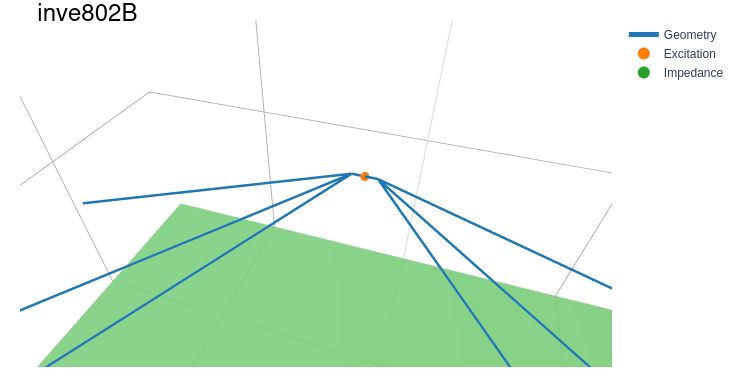
An old web-page from 1998 by Dr. Carol F. Milazzo, KP4MD has examples of antennas simulated with Mininec. The first of these examples is three crossed inverted-V (one of which has loading inductors to boost the effective length). The simulation results of pymininec are in the ballpark of the Mininec-based NEC4WIN which was used by KP4MD. But it looks like NEC4WIN might use what it prints as "Diam." as the radius of the wire (see Fig. 1 in the website) as the radius (see Antenna Model Files in the Appendix). At least if this format is inherited from NEC the last column of the wire definition would hold the radius and this interpretation of the format also is more consistent with the simulation results of Pymininec. The following table shows the original data compared to using half of the diameter in the original model in Pymininec ("Pymininec r") and the diameter as the radius (Pymininec 2r). When using the (supposed) diameter for the radius, the output data matches better to the website data.
| Frequency | Original | Pymininec r | Pymininec 2r | |
| 7MHz | Gain Azimuth | -2.42 dBi | -2.52 dBi | -2.49 dBi |
| Gain Elevation | 7.21 dBi | 7.21 dBi | 7.21 dBi | |
| Impedance | 38.74 +6.77j | 38.82 -3.66j | 39.28 +1.49j | |
| 14MHz | Gain Azimuth | 4.33 dBi | 4.60 dBi | 4.37 dBi |
| Gain Elevation | 7.23 dBi | 7.73 dBi | 7.38 dBi | |
| Impedance | 46.16 -326j | 31.86 -307j | 43.00 -313j |
All of KP4MD's examples have been converted to Pymininec and are available as
inve802B.pym, hloop40-14.pym, hloop40-7.pym,
vloop20.pym, and lzh20.pym in the test directory. Only the
inve802B.pym (with the inverted-Vs) uses the diameter in the
original example as the radius in Pymininec, all others use half of the
value in the original example (which is supposed to be the diameter) as
the radius. But most examples match better to the values computed by
KP4MD when doubling the radius.
There are some new tests that check the feedpoint impedance against known computations from the literature. In particular an old article by Roy Lewallen [8] with the same title as this section.
The column "Python" is from pymininec, the column "Basic Yabasi" is the original Basic implementation run with my Basic interpreter Yabasi. The column "Basic pcbasic" uses the pcbasic interpreter.
Note that the "Bent Dipole" is bent horizontally (not an inverted V),
all wire ends are the same height. I have not been able so far to
reproduce the results of the special segmentation scheme that uses only
14 segements with the same results as indicated in the article (see then
entry 14* for the bent dipole). When trying to reproduce it exactly
the imaginary part is much lower (more capacity). The segmentation
scheme is also not very good: In mininec adjacent segment should only
have a factor of 2 in length, not more. The segmentation special scheme
has a jump of factor 5, maybe this makes it numerically instable so that
we get much different results with double precision float.
For the bent dipole I've made three more experiments: One with tapering
from both ends (entry 14t2) and two with tapering from one end (entry
14t1 and 14t1l). Example 14t1 has no limit on segment length
while entry 14t1l enforces a minimum segment length of 1/200 lambda.
In all the cases where tapering is from one end, the end with the
feedpoint has the smallest segment length. None of these experiments
comes close to the 14 segment experiment in the paper.
| Segs | Lewallen | Python | Basic Yabasi | Basic pcbasic |
| 10 | 74.073+20.292j | 74.074+20.298j | 74.074+20.298j | 74.074+20.300j |
| 20 | 75.870+21.877j | 75.872+21.897j | 75.872+21.897j | 75.872+21.897j |
| 30 | 76.573+23.218j | 76.567+23.169j | 76.567+23.169j | 76.572+23.203j |
| 40 | 76.972+24.053j | 76.972+24.052j | 76.972+24.052j | 76.973+24.068j |
| 50 | 77.222+24.517j | 77.240+24.647j | 77.240+24.647j |
| Segs | Lewallen | Python | Basic Yabasi | Basic pcbasic |
| 10 | 11.509-76.933j | 11.498-77.045j | 11.498-77.045j | 11.498-77.044j |
| 20 | 11.751-53.812j | 11.740-53.929j | 11.740-53.929j | 11.740-53.932j |
| 30 | 11.819-46.934j | 11.808-47.068j | 11.808-47.068j | 11.808-47.055j |
| 40 | 11.848-43.783j | 11.837-43.893j | 11.837-43.893j | 11.838-43.858j |
| 50 | 11.861-41.988j | 11.851-42.107j | 11.851-42.107j | |
| 14* | 11.312-43.119j | 11.104-47.879j | ||
| 14t1 | 10.859-42.486j | |||
| 14t1l | 11.118-46.593j | |||
| 14t2 | 11.314-45.659j | |||
You can run the tests with:
python3 -m pytest test
If coverage should be reported this becomes:
python3 -m pytest --cov mininec test
For a more detailed coverage report use:
python3 -m pytest --cov-report term-missing --cov mininec test
This will show a detailed report of the lines that are not covered by tests.
[This section uses math in ReStructuredText which may not render correctly on all platforms. In particular, Github has an open issue on this for more than a decade now. It is said to be supported on pypi, let's see.]
To support skin effect loads on geometry objects (e.g. wires) we need to compute the internal impedance of a segment. The Wikipedia article on skin effect has the following formula for the internal impedance per unit length:
\newcommand{\Int}{{\mathrm\scriptscriptstyle int}}
\newcommand{\ber}{\mathop{\mathrm{ber}}\nolimits}
\newcommand{\bei}{\mathop{\mathrm{bei}}\nolimits}
Z_\Int = \frac{k\rho}{2\pi r}\frac{J_0 (kr)}{J_1 (kr)}
where
k = \sqrt{\frac{-j\omega\mu}{\rho}}
and r is the radius, J_v are the Bessel functions of the first kind of order v. Z_\Int is the impedance per unit length of wire.
Since the Wikipedia article on skin effect cites this from a book not available to me, I've looked in a classic, Chipman's Theory and Problems of Transmission Lines [9]. This has the following formula for Z_\Int (6.27 p.77):
Z_\Int = \frac{jR_s}{\sqrt{2}\pi a}
         \frac{\ber(\sqrt{2}a/\delta) + j\bei(\sqrt{2}a/\delta)}
         {\ber^\prime(\sqrt{2}a/\delta) + j\bei^\prime(\sqrt{2}a/\delta)}
with
R_s = \frac{1}{\sigma\delta} = \sqrt{\frac{\omega\mu}{2\sigma}}
and \delta the skin depth (in formula 6.15, p. 74):
\delta = \sqrt{\frac{2}{\omega\mu\sigma}}
and a the radius. Note that this formula is identical to the formula used by the Fortran implementation of NEC-2 as derived in my blog post [10]. But it is not identical to the one described in the theoretical paper on NEC [11] (p. 75) which is wrong as shown in my blog post [10].
Chipman [9] also has a conversion from the Kelvin functions to the Bessel functions (formula 6.11 and 6.12 on p. 74):
\ber (x) = \Re (J_0(\sqrt{-j}x)) \\
\bei (x) = \Im (J_0(\sqrt{-j}x)) \\
with \Re being the real part and \Im being the imaginary part of a complex number. In one expression this is:
J_0 \left(\sqrt{-j}x\right) = \ber (x) + j\bei(x)
For the derivative we have:
-J_1 \left(\sqrt{-j}x\right) \sqrt{-j} = \ber^\prime(x) + j\bei^\prime(x)
and consequently for the fraction of Kelvin functions:
\frac{\ber (x) + j\bei(x)}{\ber^\prime(x) + j\bei^\prime(x}
= \frac{-1}{\sqrt{-j}}\frac{J_0(\sqrt{-j}x)}{J_1(\sqrt{-j}x}
Replacing this into the Z_\Int formula above we get:
Z_\Int = \frac{-jR_s}{\sqrt{2}\pi a}
         \frac{1}{\sqrt{-j}}
         \frac{J_0(\sqrt{-2j}a/\delta)}{J_1(\sqrt{-2j}a/\delta)}
Making use of the fact that
\sqrt{-j} = \frac{1-j}{\sqrt{2}}
we get
Z_\Int =& \frac{-jR_s}{(1-j)\pi a}
          \frac{J_0((1-j)a/\delta)}{J_1((1-j)a/\delta)} \\
       =& \frac{(1-j)R_s}{2\pi a}
          \frac{J_0((1-j)a/\delta)}{J_1((1-j)a/\delta)} \\
replacing R_s and \delta and using \rho=1/\sigma we get
Z_\Int = \frac{(1-j)}{2\pi a}
         \sqrt{\frac{\omega\mu\rho}{2}}
         \frac{J_0\left((1-j)a\sqrt{\frac{\omega\mu}{2\rho}}\right)}
              {J_1\left((1-j)a\sqrt{\frac{\omega\mu}{2\rho}}\right)}
substituting k above and using
\sqrt{-2j} = (1-j)
k = \sqrt{\frac{-j\omega\mu}{\rho}}
Z_\Int =& \frac{(1-j)k}{2\pi a}
          \sqrt{\frac{\rho^2}{-2j}}
          \frac{J_0\left(\frac{(1-j)ak}{\sqrt{-2j}}\right)}
               {J_1\left(\frac{(1-j)ak}{\sqrt{-2j}}\right)} \\
       =& \frac{k\rho}{2\pi a} \frac{J_0(ak)}{J_1(ak)} \\
which is identical to the Wikipedia formula when we substitute a=r. This is the formula that is used for skin effect loads in pymininec.
A note on the history of using Kelvin functions instead of Bessel functions here: Before the age of pocket calculators there were ready-made tables for Kelvin functions. Lookup of complex arguments to functions via tables was not possible, so a solution that was computable with books of mathematical tables was preferred...
Insulated wires use a distributed inductance and equivalent radius:
a_e &= a \left(\frac{b}{a}\right)^{\left(1-
    \frac{1}{\varepsilon_r}\right)}
    = b \left(\frac{a}{b}\right)^\left(\frac{1}{\varepsilon_r}\right) \\
L   &= \frac{\mu_0}{2\pi}\left(1-\frac{1}{\varepsilon_r}
  \right)\log\left(\frac{b}{a}\right) \\
where a is the original radius of the wire, b is the radius of the wire including insulation, \varepsilon_r is the relative dieelectric constant of the insulation, \mu_0 is the vacuum permeability, and a_e is the equivalent radius. The inductance L is the inductance per length of the insulated wire (or wire segment).
This formula originally appeared in a paper by Wu [12]. I discovered it via a note by Steve Stearns, K6OIK which turned out to be a supplement to the ARRL Antenna Book [13].
I had first tried a formulation by Richmond [15] suggested to me by Roy Lewallen, W7EL (the author of EZNEC). But that formulation turned out to be numerically instable for small segments. More details are in my blog [16].
The Mininec code uses the implementation of an elliptic integral when computing the impedance matrix and in several other places. The integral uses a set of E-vector coefficients that are cited differently in different places. In the latest version of the open source Basic code these parameters are in lines 1510–1512. They are also reprinted in the publication [2] about that version of Mininec which has a listing of the Basic source code (slightly different from the version available online) where it is on p. C-31 in lines 1512–1514.
| 1.38629436112 | .09666344259 | .03590092383 | .03742563713 | .01451196212 |
| .5 | .12498593397 | .06880248576 | .0332835346 | .00441787012 |
In one of the first publications on Mininec [1] the authors give the parameters on p. 13 as:
| 1.38629436112 | .09666344259 | .03590092383 | .03742563713 | .01451196212 |
| .5 | .1249859397 | .06880248576 | .03328355346 | .00441787012 |
This is consistent with the later Mininec paper [2] on version 3 of the Mininec code on p. 9, but large portions of that paper are copy & paste from the earlier paper.
The first paper [1] has a listing of the Basic code of that version and on p. 48 the parameters are given as:
| 1.38629436 | .09666344 | .03590092 | .03742563713 | .01451196 |
| .5 | .12498594 | .06880249 | .0332836 | .0041787 |
In each case the first line are the a parameters, the second line are the b parameters. The a parameters are consistent in all versions but notice how in the b parameters (2nd line) the current Basic code has one more 3 in the second column. The rounding of the earlier Basic code suggests that the second 3 is a typo in the later Basic version. Also notice that in the 4th column the later Basic code has a 5 less than the version in the papers. The rounding in the earlier Basic code also suggests that the later Basic code is in error.
The errors in the elliptic integral parameters do not have much effect on the computed values of the Mininec code. There are some minor differences but these are below the differences between Basic and Python implementation (single vs. double precision arithmetics). I had hoped that this has something to do with the well known fact that Mininec finds a resonance point of an antenna some percent too high which means that usually in practice the computed wire lengths are a little too long. This is apparently not the case. The resonance point is also wrong for very thin wires below the small radius modification condition which happens when the wire radius is below 1e-4 of the wavelength. Even in that case – where the elliptic integral is not used – the resonance is slightly wrong.
The reference for the elliptic integral parameters [3] cited in both reports lists the following table on p. 591:
| 1.38629436112 | .09666344259 | .03590092383 | .03742563713 | .01451196212 |
| .5 | .12498593597 | .06880248576 | .03328355346 | .00441787012 |
Note that I could only locate the 1972 version of the Handbook, not the 1980 version cited by the reports. So there is a small chance that these parameters were corrected in a later version. It turns out that the reports are correct in the fourth column and the Basic program is wrong. But the second column contains still another version, note that there is a 5 in the 9th position after the comma, not a 3 like in the Basic program and not a missing digit like in the Mininec reports [1] [2].
Since I could not be sure that there was a typo in the handbook [3], I dug deeper: The handbook cites Approximations for Digital Computers by Hastings (without giving a year) [4]. The version of that book I found is from 1955 and lists the coefficients on p. 172:
| 1.38629436112 | .09666344259 | .03590092383 | .03742563713 | .01451196212 |
| .5 | .12498593597 | .06880248576 | .03328355346 | .00441787012 |
So apparently the handbook [3] is correct. And the Basic version and both Mininec reports have at least one typo.
Since this paragraph was written the implementation of the elliptic
integral was removed and replace with a call to scipy.special.ellipk.
The resulting differences in computed outputs were smaller than the
differences between the Basic (single precision) and the Python (double
precision) implementation.
The original Basic source code can still be run today.
Thanks to Rob Hagemans pcbasic project I had a starting point for debugging the initial pymininec implementation. It is written in Python and can be installed with pip. It is also packaged in some Linux distributions, e.g. in Debian.
In the meanwhile I've written my own Basic interpreter over a weekend called Yabasi for two reasons:
- pcbasic faithfully reproduces the memory limitations of the time
- pcbasic does some effort to compute in single precision float numbers
A third reason materialized when I had Yabasi working: It is much faster than pcbasic.
Since Mininec reads all inputs for an antenna simulation from the
command-line in Basic, I'm creating input files that contain
reproduceable command-line input for an antenna simulation. An example
of such a script is in dipole-01.mini, the suffix mini
indicating a Mininec file. These can be directly run with Yabasi (using
the -i option), for running with pcbasic they need to be converted
to carriage-return line endings. The Makefile has code for this, you can
run, e.g.:
make vertical-rad.CR
and a carriage-return version of test/vertical-rad.mini will be
created.
Of course the input files only make sense if you actually run them with the mininec basic code as this displays all the prompts. Note that I had to change the dimensions of some arrays in the Basic code to not run into an out-of-memory condition with the pcbasic Basic interpreter.
You can run pcbasic with the command-line option --input= to specify
an input file. Note that the input file has to be converted to carriage
return line endings (no newlines). I've described how I'm debugging the
Basic code using the Python debugger in a contribution to pcbasic,
this has been moved to the pcbasic wiki.
For Yabasi this debugging is built-in, you can specify the command-line
option -L <line> where <line> is the line number in the Basic
code where you want to stop. When stopped you can set
!self.break_lineno = 'all'
to single step through the Basic program. Alternatively you can specify another line number you want to stop at.
In the file debug-basic.txt you can find my notes on how to debug
mininec using the python debugger with pcbasic. This is more or less a
random cut&paste buffer.
The original basic source code used to be at the unofficial NEC archive by PA3KJ or from the Mininec github project by the same author, the unofficial NEC archive site seems to experience problems (empty page) as of this writing.
I have a patched MININEC version on github that forks the Mininec github project and does some small fixes that:
- use larger
DIMstatements - fixes elliptic integral parameters and uses better accuracy for elliptic curve and gaussian quadrature parameters
- Uses a better accuracy of the hard-coded constand 1/log(10)*10 which is used during far field computation (to get dBi). This makes the MININEC results of the far field better match the python implementation.
My MININEC version cannot be run with pcbasic because the DIM statements use too much memory.
v1.1: Feature improvements
- Lay the groundwork for implementation of further geometry objects not just wires
- Wires (and future geometry objects) can have tags, all usage of wires, segments, pulses, and loads now use a tag which is a 1-based auto-computed number which can be explicitly specified for wires; the tag is used in all error messages
- Add segment length tapering: Wires can now be split into segments of unequal length
- Add skin effect loads
- Add insulated wire loads
- Add geometry transformations rotation, translation, and scaling
- Implement round-tripping of command-line parameters, allow to output the current settings as command-line options
- Implement output of the Basic input to test an antenna model against the original Basic implementation
- The
--excitation-segmentoption has been renamed to--excitation-pulseand it now allows specification of the pulse relative to a geometry object (e.g. wire)
v1.0: Speed improvement by vectorization
- Vectorize far field computation
- Vectorize computation of the impedance matrix
- Vectorize near field computation
v0.6.1: Fix entry point for script
v0.6.0: Add pyproject.toml
- Add pyproject.toml
- Add LICENSE file
- Minor fixes
v0.5.0: Bug fixes and new load types
- New load types RLC load and Trap load: The first uses a series R-L-C (with each being optional), the second serial R-L parallel to a C (for a good emulation of traps in antennas)
- Bug-Fix in wire-end matching: If there are multiple wires connected to a single point the previous implementation would not build the data structures correctly
- Add more regression tests
- Get rid of unittest to avoid a mixture of the unittest and pytest testing frameworks
v0.4.0: Split plot-antenna into own project
- Own project plot-antenna
- Fix parsing of several medium options, mention ground in documentation
v0.3.0: Laplace loads correctly implemented
- Use scipy.special.ellipk for elliptic integral
- Use gaussian quadrature coefficients from scipy.integrate
- Test resonance (NEC vs. mininec)
v0.2.0: Add short paragraph on new plotting program
- Test coverage
- Expression simplification
v0.1.0: Initial release
| [1] | (1, 2, 3) Alfredo J. Julian, James C. Logan, and John W. Rockway. Mininec: A mini-numerical electromagnetics code. Technical Report NOSC TD 516, Naval Ocean Systems Center (NOSC), San Diego, California, September 1982. Available as ADA121535 from the Defense Technical Information Center. |
| [2] | (1, 2, 3, 4) J. C. Logan and J. W. Rockway. The new MININEC (version 3): A mini-numerical electromagnetic code. Technical Report NOSC TD 938, Naval Ocean Systems Center (NOSC), San Diego, California, September 1986. Available as ADA181682 from the Defense Technical Information Center. Note: The scan of that report is very bad. If you have access to a better version, please make it available! |
| [3] | (1, 2, 3) Milton Abramowitz and Irene A. Stegun, editors. Handbook of Mathematical Functions With Formulas, Graphs, and Mathematical Tables. Number 55 in Applied Mathematics Series. National Bureau of Standards, 1972. |
| [4] | Cecil Hastings, Jr. Approximations for Digital Computers. Princeton University Press, 1955. |
| [5] | (1, 2) Rafik Paul Zeineddin. Numerical electromagnetics codes: Problems, solutions and applications. Master’s thesis, Ohio University, March 1993. Available from the OhioLINK Electronic Theses & Dissertations Center |
| [6] | (1, 2) L. B. Cebik. Radiation plots: Polar or rectangular; log or linear. In Antenna Modeling Notes [7], chapter 48, pages 366–379. Available in Cebik's Antenna modelling notes episode 48 |
| [7] | L. B. Cebik. Antenna Modeling Notes, volume 2. antenneX Online Magazine, 2003. Available with antenna models from the Cebik collection. |
| [8] | Roy Lewallen. Mininec: The other edge of the sword. QST, pages 18–22, February 1991. |
| [9] | (1, 2) Robert A. Chipman. Theory and Problems of Transmission Lines. Schaums Outline. McGraw-Hill, 1968. |
| [10] | (1, 2) Ralf Schlatterbeck. Skin Effect Load Update. Blog post, Open Source Consulting, July 2024. |
| [11] | (1, 2) G. J. Burke and A. J. Poggio. Numerical electromagnetics code (NEC) – method of moments, Part I: Program description – theory. January 1981. |
| [12] | Tai Tsun Wu. Theory of the dipole antenna and the two-wire transmission line. Journal of Mathematical Physics, 2(4):550–574, July 1961. |
| [13] | Steve Stearns. Modeling insulated wire. In Silver [11]. Supplement to Antenna Book, page visited 2024-08-26. |
| [14] | H. Ward Silver, editor. The ARRL Antenna Book for Radio Communications. American Radio Relay League (ARRL), 25th edition, 2023. |
| [15] | J. H. Richmond. Radiation and scattering by thin-wire structures in the complex frequency domain. Contractor Report CR-2396, NASA, Columbia, Ohio, May 1974. Available as CR-2936 |
| [16] | Ralf Schlatterbeck. Modeling a wire antenna with insulation. Blog post, Open Source Consulting, September 2024. |