rgamer

Overview

The goal of rgamer is to help students learn Game Theory using R. The functions prepared by the package not only solve basic games such as two-person normal-form games but also provides the users with visual displays that highlight some aspects of the games — payoff matrix, best response correspondence, etc. In addition, it suggests some numerical solutions for games of which it is difficult — or even seems impossible — to derive a closed-form analytical solution.

Installation

You can install the development version from GitHub with:

# install.packages("remotes")
remotes::install_github("yukiyanai/rgamer")

# install.packages("devtools")
devtools::install_github("yukiyanai/rgamer")

Examples

library(rgamer)

Example 1

An example of a normal-form game (prisoner’s dilemma).

Player: {Kamijo, Yanai }
Strategy: {(Stays silent, Betrays), (Stays silent, Betrays)}
Payoff: {(-1, 0, -3, -2), (-1, -3, 0, -2)}

First, you define the game by normal_form():

game1 <- normal_form(
  players = c("Kamijo", "Yanai"),
  s1 = c("Stays silent", "Betrays"), 
  s2 = c("Stays silent", "Betrays"), 
  p1 = c(-1,  0, -3, -2), 
  p2 = c(-1, -3,  0, -2))

Then, you can pass it to solve_nfg() function to get the table of the game and the Nash equilibrium.

s_game1 <- solve_nfg(game1)

#> Pure-strategy NE: (Betrays, Betrays)

Example 2

An example of a coordination game.

Player: {Kamijo, Yanai }
Strategy: {(Stag, Hare), (Stag, Hare)}
Payoff: {(10, 8, 0, 7), (10, 0, 8, 7)}

Define the game by normal_form():

game2 <- normal_form(
  players = c("Kamijo", "Yanai"),
  s1 = c("Stag", "Hare"), 
  s2 = c("Stag", "Hare"), 
  p1 = c(10, 8, 0, 7), 
  p2 = c(10, 0, 8, 7))

Then, you can pass it to solve_nfg() function to get NEs. Set mixed = TRUE to find mixed-strategy NEs well.

s_game2 <- solve_nfg(game2, mixed = TRUE, show_table = FALSE)
#> Pure-strategy NE: (Stag, Stag)(Hare, Hare)
#> Mixed-strategy NE: [(7/9, 2/9), (7/9, 2/9)]
#> The obtained mixed-strategy NE might be only a part of the solutions.
#> Please examine br_plot (best response plot) carefully.

For a 2-by-2 game, you can plot the best response correspondences as well.

s_game2$br_plot

Example 3

An example of a normal-form game:

Player: { A, B }
Strategy: {x ∈ [0, 30], y ∈ [0, 30] }
Payoff: {f_x(x, y) = − x² + (28 − y)x, f_y(x, y) = − y² + (28 − x)y}

You can define a game by specifying payoff functions as character vectors using normal_form():

game3 <- normal_form(
  players = c("A", "B"),
  p1 = "-x^2 + (28 - y) * x",
  p2 = "-y^2 + (28 - x) * y",
  par1_lim = c(0, 30),
  par2_lim = c(0, 30),
  pars = c("x", "y"))

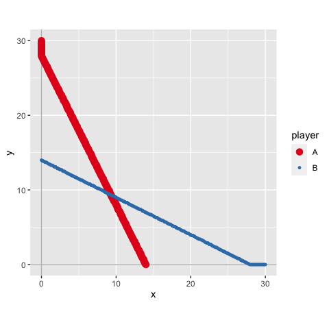
Then, you can pass it to solve_nfg(), which displays the best response correspondences by default.

s_game3 <- solve_nfg(game3)
#> approximated NE: (9.3, 9.3)
#> The obtained NE might be only a part of the solutions.
#> Please examine br_plot (best response plot) carefully.

Example 4

An example of a normal-form game:

Player: { A, B }
Strategy: {x ∈ [0, 30], y ∈ [0, 30] }
Payoff: {f_x(x, y) = − x^a + (b − y)x, f_y(x, y) = − y^s + (t − x)y}

You can define a normal-form game by specifying payoffs by R functions.

f_x <- function(x, y, a, b) {
  -x^a + (b - y) * x
}
f_y <- function(x, y, s, t) {
  -y^s + (t - x) * y
}
game4 <- normal_form(
  players = c("A", "B"),
  p1 = f_x,
  p2 = f_y,
  par1_lim = c(0, 30),
  par2_lim = c(0, 30),
  pars = c("x", "y"))

Then, you can approximate a solution numerically by solve_nfg(). Note that you need to set the parameter values of the function that should be treated as constants by arguments cons1 and cons2, each of which accepts a named list. In addition, you can suppress the plot of best responses by plot = FALSE.

s_game4 <- solve_nfg(
  game = game4,
  cons1 = list(a = 2, b = 28),
  cons2 = list(s = 2, t = 28),
  plot = FALSE)
#> approximated NE: (9.3, 9.3)
#> The obtained NE might be only a part of the solutions.
#> Please examine br_plot (best response plot) carefully.

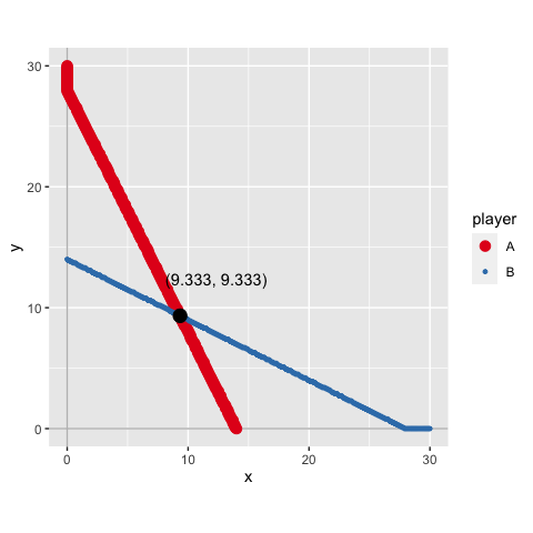
You can increase the precision of approximation by precision, which takes a natural number (default is precision = 1).

s_game4b <- solve_nfg(
  game = game4,
  cons1 = list(a = 2, b = 28),
  cons2 = list(s = 2, t = 28),
  precision = 3)
#> approximated NE: (9.333, 9.333)
#> The obtained NE might be only a part of the solutions.
#> Please examine br_plot (best response plot) carefully.

You can extract the best response plot with NE marked as follows.

s_game4b$br_plot_NE

Example 5

You can define payoffs by R functions and evaluate them at some discretized values by setting discretize = TRUE. The following is a Bertrand competition example:

func_price1 <- function(p, q) {
  if (p < q) {
    profit <- p
  } else if (p == q) {
    profit <- 0.5 * p
  } else {
    profit <- 0
  }
  profit
}

func_price2 <- function(p, q){
  if (p > q) {
    profit <- q
  } else if (p == q) {
    profit <- 0.5 * q
  } else {
    profit <- 0
  }
  profit
}

game5 <- normal_form(
  p1 = func_price1,
  p2 = func_price2,
  pars = c("p", "q"),
  par1_lim = c(0, 10),
  par2_lim = c(0, 10),
  discretize = TRUE)

Then, you can examine the specified part of the game.

s_game5 <- solve_nfg(game5, mark_br = FALSE)

#> Pure-strategy NE: (0, 0)(2, 2)(4, 4)

Example 6

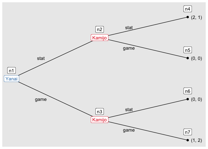
You can draw a tree of an extensive form game.

game6 <- extensive_form(
  players = list("Yanai", 
                 rep("Kamijo", 2),
                 rep(NA, 4)),
  actions = list(c("stat", "game"),
                  c("stat", "game"), c("stat", "game")),
  payoffs = list(Yanai = c(2, 0, 0, 1),
                 Kamijo = c(1, 0, 0, 2)),
  direction = "right")

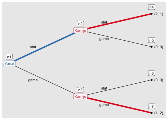
And you can find the solution of the game by solve_efg().

s_game6 <- solve_efg(game6)
#> backward induction: [(stat), (stat, game)]

Then, you can see the path played under a solution by show_path().

show_path(s_game6)

schoulten/rgamer