By Abhinav M. Hari, Ramya Iyer, Venkata Menta and Daniel Wang
You might’ve heard all sorts of analogies trying to explain what superposition is. Whether it’s a cat in a box that’s both alive and dead (i.e. Schrödinger's cat), a flipped coin that’s both heads and tails, or an electron in both spin up and spin down, quantum superposition is definitely a strange and fascinating topic.
 |
 |
|---|---|
| Courtesy of Wikipedia | Courtesy of Chemistry God |
This article assumes that you have a basic understanding of what quantum superposition is. Moreover, we will dive into the basic mathematical representations of quantum superposition. Although it is not an extensive overview, it does give a basic understanding of how linear algebra is used in quantum computing.
Quantum superposition is one of the three quantum phenomenons that enable quantum computers to compute in ways classical computers cannot.
A technical explanation for quantum superposition is that a quantum system (i.e. a qubit) can exist in a quantum state (i.e. |0> or |1>) and a linear combination of multiple quantum states.
Let’s break down that definition just a little bit.
So what exactly is a quantum system? Well in quantum computing, our quantum system is a qubit, the quantum version of a classical bit which can be found in your regular classical computer.
(We won’t worry too much about the physical implementation of a qubit in this article, because there are a variety of different ways to build a qubit.)
Since superposition allows for a qubit to be in two states simultaneously (|0> and |1> at the same time), n qubits will represent 2n quantum states. This allows for an exponential increase in complexity: 1 qubit can simultaneously represent 2 quantum states, 2 qubits 4 quantum states, 3 qubits 8 quantum states, 4 qubits 16 quantum states, and so on.
This differs from classical bits where each additional bit only increases the complexity by 2, thus n bits will represent 2n binary states.
This exponential increase derived from superposition, allows quantum computers to solve some complex problems that would be impossible for classical computers to do in a reasonable time period.
Now let’s talk about quantum states.
Similar to how a binary bit can be a 0 or 1, a qubit can be in the quantum states |0> or |1>, (the | > notation is called bra-ket notation and it signifies that we are dealing with values in the quantum realm).
In addition to the quantum states being |0> or |1>, there exists a quantum state that’s in a superposition, a linear combination of |0> and |1>, denoted as |ψ>.
We can represent |ψ> mathematically by the following equation. (Don’t get too scared of the greek letters, we’ll be explaining them!)
|ψ> = α|0> + β|1>
Let’s break this equation down even further.
α|0> → α is the probability coefficient of the quantum state |0>, which must be between -1 and 1.
Squaring the absolute value of α, |α|2, will give you the probability of the superposition collapsing to the quantum state |0> when it is measured.
Before a qubit is measured, it “stays” quantum, meaning that it is still able to exhibit the quantum property of superposition. However after it is measured the qubit “collapses” into the state 0 or 1, and no longer exhibits quantum properties. One could say that after a qubit is measured, it turns from a quantum bit to a classical bit.
β|1> → β is a coefficient that contains the same rules as α except it pertains to the quantum state |1>.
Similarly, |β|2 results in the probability of the superposition collapsing in the quantum state |1> when it is measured.
Intuitively, |α|2 + |β|2 = 1 because there is a 100% probability you will get either the state |0> or |1> after measurement.
This equation shows a new quantum state (|ψ>) that a quantum system (qubit) can be in where it is in a probability of being |0> or |1>, and is thus described as being both simultaneously.
We can also represent the quantum states in the form of a vector.
If we take the previous equation explained above, |ψ> = α|0> + β|1>
Representing quantum states in a vector form can be especially helpful, as linear algebra is often used to mathematically represent quantum gates (such as the Hadamard gate) being applied to qubits. (interested in learning more about linear algebra check out the resources below this article).
In quantum computing, there is a special quantum gate that creates an equal 50-50 superposition called the Hadamard Gate. This can be represented as (|0>+|1>)/√2. When the Hadamard gate is applied to |0> and |1>, we get the following outputs.
| Input | Output |
|---|---|
| |0> | (|0>+|1>)/√2 |
| |1> | (|0>-|1>)/√2 |
import qiskit as q
from qiskit import IBMQ, Aer #local simulator framework for qiskit
from qiskit.tools.monitor import job_monitor
from qiskit.visualization import plot_histogram
%matplotlib inline
from matplotlib import style

circuit = q.QuantumCircuit(1,1) # 1 qubit, 1 classical bit

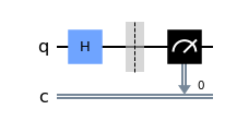
circuit.h(0) #hadamard gate --> creating an equal superposition of |0> and |1>
circuit.barrier()
circuit.measure(0,0) #measurement --> collapses the qubit

circuit.draw(output="mpl") #creates a matplotlib drawing of the gates |
|---|
| Matplotlib representation of quantum circuit |
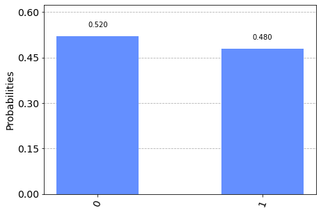
At the barrier, the qubit’s state is (|0>+|1>)/√2: an equal superposition of |0> and |1>. When measured, the state of the qubit collapses into one of the two states, |0> or |1>. Below is the code and the bar graph produced by running the circuit on an IBM machine.
backend = provider.get_backend("ibmq_belem")
job = q.execute(circuit, backend=backend, shots = 500) # we manually set the circuit to run 500 times
result = job.result()
counts = result.get_counts(circuit)
plot_histogram([counts]) # bar graph with the probability that the qubit collapsed into |0> or |1>  |
|---|
| IBM Quantum Results: 0-qubit = .520 and 1-qubit = .480, representing the probability of each occurrence |
The bar graph depicts an approximate equal superposition, which is what we expect from the Hadamard gate. (You might be wondering why it isn’t exactly .5 and .5 as we would expect: This is because this quantum circuit was run on real quantum computers. At the moment all real quantum computers have noise, resulting in some degree of inaccuracy.)
There’s a lot more math we can go into, and if you’d like to know more of the mathematical details check out the great resources in the description.
We hope that this article was informative about some of the more advanced concepts quantum superposition.
- (Video) Understanding Quantum Mechanics #2: Superposition and Entanglement by Sabine Hossenfelder
- (Video) How Does a Quantum Computer Work?: Veritasium
- (Blog) The Math behind Quantum Computing - Qubits and Superposition: Ryan Lam
- (Blog) Basic Guide to Quantum Computing and Superposition: Mark Rethana
- (Blog) Quantum Computing Series, Part 4: Superposition in Quantum Mechanics: Scott Amyx