The glmmfields R package implements Bayesian spatiotemporal models that allow for extreme spatial deviations through time. It uses a predictive process approach with random fields implemented through a multivariate-t distribution instead of a multivariate normal. The models are fit with Stan.
We published a paper describing the model and package in Ecology:
Anderson, S. C., Ward, E. J. 2019. Black swans in space: modelling spatiotemporal processes with extremes. 100(1):e02403. https://doi.org/10.1002/ecy.2403
You can install the CRAN version of the package with:
install.packages("glmmfields")If you have a C++ compiler installed, you can install the development version of the package with:
# install.packages("remotes")
remotes::install_github("seananderson/glmmfields", build_vignettes = TRUE)
glmmfields can also fit spatial GLMs with Stan. See the vignette:
vignette("spatial-glms", package = "glmmfields")library(glmmfields)
#> Loading required package: Rcpp
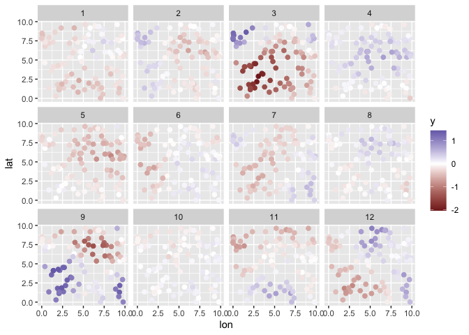
library(ggplot2)Simulate data:
set.seed(42)
s <- sim_glmmfields(
  df = 2.8, n_draws = 12, n_knots = 12, gp_theta = 2.5,
  gp_sigma = 0.2, sd_obs = 0.1
)
head(s$dat)
#>   time pt           y      lon      lat station_id
#> 1    1  1  0.02818963 9.148060 6.262453          1
#> 2    1  2 -0.21924739 9.370754 2.171577          2
#> 3    1  3 -0.34719485 2.861395 2.165673          3
#> 4    1  4 -0.15785483 8.304476 3.889450          4
#> 5    1  5 -0.04703617 6.417455 9.424557          5
#> 6 1 6 -0.23904924 5.190959 9.626080 6print(s$plot)Fit the model:
options(mc.cores = parallel::detectCores()) # for parallel processing
m <- glmmfields(y ~ 0,
  data = s$dat, time = "time",
  lat = "lat", lon = "lon",
  nknots = 12, estimate_df = TRUE, iter = 800, seed = 1
)print(m)
#> Inference for Stan model: glmmfields.
#> 4 chains, each with iter=800; warmup=400; thin=1;
#> post-warmup draws per chain=400, total post-warmup draws=1600.
#>
#> mean se_mean sd 2.5% 25% 50% 75% 97.5% n_eff Rhat
#> df[1] 3.72 0.04 1.47 2.08 2.67 3.37 4.28 7.48 1331 1
#> gp_sigma 0.30 0.00 0.04 0.22 0.27 0.30 0.32 0.39 525 1
#> gp_theta 2.58 0.00 0.07 2.46 2.54 2.58 2.63 2.71 1434 1
#> sigma[1] 0.10 0.00 0.00 0.09 0.10 0.10 0.10 0.10 2207 1
#> lp__ 2291.28 0.42 9.59 2270.34 2285.12 2291.59 2297.73 2308.74 521 1
#>
#> Samples were drawn using NUTS(diag_e) at Mon Feb 13 12:45:42 2023.
#> For each parameter, n_eff is a crude measure of effective sample size,
#> and Rhat is the potential scale reduction factor on split chains (at
#> convergence, Rhat=1).Plot:
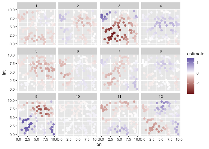
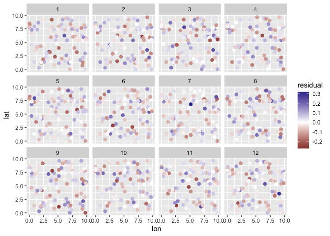
plot(m, type = "prediction") + scale_color_gradient2()plot(m, type = "spatial-residual")Predictions:
# link scale:
p <- predict(m)
head(p)
#> # A tibble: 6 × 3
#>   estimate conf_low conf_high
#>      <dbl>    <dbl>     <dbl>
#> 1  -0.0283  -0.0868    0.0273
#> 2  -0.291   -0.365    -0.220
#> 3  -0.397   -0.448    -0.346
#> 4  -0.196   -0.266    -0.123
#> 5  -0.0370  -0.110     0.0360
#> 6  -0.214   -0.294    -0.140

# posterior predictive intervals on new observations (include observation error):
p <- predictive_interval(m)
head(p)
#> # A tibble: 6 × 3
#>   estimate conf_low conf_high
#>      <dbl>    <dbl>     <dbl>
#> 1  -0.0283   -0.236   0.181
#> 2  -0.291    -0.507  -0.0904
#> 3  -0.397    -0.596  -0.206
#> 4  -0.196    -0.392   0.00154
#> 5  -0.0370   -0.239   0.172
#> 6  -0.214    -0.423  -0.00659
Use the tidy method to extract parameter estimates as a data frame:
x <- tidy(m, conf.int = TRUE)
head(x)
#> # A tibble: 6 × 5
#>   term                     estimate std.error conf.low conf.high
#>   <chr>                       <dbl>     <dbl>    <dbl>     <dbl>
#> 1 df[1]                      3.37     1.47      2.08      7.48
#> 2 gp_sigma                   0.295    0.0432    0.216     0.388
#> 3 gp_theta                   2.58     0.0662    2.46      2.71
#> 4 sigma[1]                   0.0979   0.00214   0.0939    0.102
#> 5 spatialEffectsKnots[1,1]  -0.110    0.0341   -0.175    -0.0442
#> 6 spatialEffectsKnots[2,1]  -0.230    0.0386   -0.305    -0.155
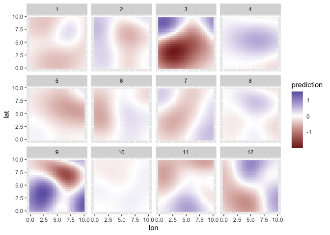
Make predictions on a fine-scale spatial grid:
pred_grid <- expand.grid(
  lat = seq(min(s$dat$lat), max(s$dat$lat), length.out = 25),
  lon = seq(min(s$dat$lon), max(s$dat$lon), length.out = 25),
  time = unique(s$dat$time)
)

pred_grid$prediction <- predict(m,
  newdata = pred_grid, type = "response", iter = 100, estimate_method = "median"
)$estimate

ggplot(pred_grid, aes(lon, lat, fill = prediction)) +
  facet_wrap(~time) +
  geom_raster() +
scale_fill_gradient2()Anderson, S. C., Ward, E. J. 2019. Black swans in space: modelling spatiotemporal processes with extremes. 100(1):e02403. https://doi.org/10.1002/ecy.2403
Latimer, A. M., S. Banerjee, H. Sang Jr, E. S. Mosher, and J. A. Silander Jr. 2009. Hierarchical models facilitate spatial analysis of large data sets: a case study on invasive plant species in the northeastern United States. Ecology Letters 12:144–154.
Shelton, A. O., J. T. Thorson, E. J. Ward, and B. E. Feist. 2014. Spatial semiparametric models improve estimates of species abundance and distribution. Canadian Journal of Fisheries and Aquatic Sciences 71:1655–1666.
This repository is a scientific product and is not official communication of the National Oceanic and Atmospheric Administration, or the United States Department of Commerce. All NOAA GitHub project code is provided on an ‘as is’ basis and the user assumes responsibility for its use. Any claims against the Department of Commerce or Department of Commerce bureaus stemming from the use of this GitHub project will be governed by all applicable Federal law. Any reference to specific commercial products, processes, or services by service mark, trademark, manufacturer, or otherwise, does not constitute or imply their endorsement, recommendation or favoring by the Department of Commerce. The Department of Commerce seal and logo, or the seal and logo of a DOC bureau, shall not be used in any manner to imply endorsement of any commercial product or activity by DOC or the United States Government.
