README.Rmd

Ça va, CAVA? Dictionary Coherence, Augmentation, (Validation and Analysis)

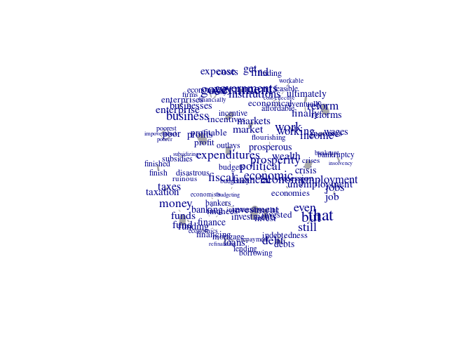
CAVA is an R package to assit in working with dictionary (keywords/lexical text analysis) in a valid way. It allows you to use an embeddings model to do dictionary expansion/augmentation, check its coherence, (and at some future date) validation and analysis.

For a longer description, see our ICA Tool Demo abstract.

Installing and obtaining an embeddings model

You can install CAVA from github:

remotes::install_github("vanatteveldt/CAVA")

Before starting, you need an embeddings model. Currently, we only support Fasttext .bin models. The code below downloads an English fasttext model:

if (!file.exists("cc.en.300.bin")) {
  url = "https://dl.fbaipublicfiles.com/fasttext/vectors-crawl/cc.en.300.bin.gz"
  options(timeout=4300)  # assuming 1Mb/s
  download.file(paste0(url), destfile = "cc.en.300.bin.gz")
  R.utils::gunzip("cc.en.300.bin.gz") # Install R.utils if needed
}

Using CAVA

The main functions exposed to cava are shown below. For a more elaborate example, please see the example usage file.

Loading the FastText mnodel, using the state of the union speeches as target corpus:

library(CAVA)
corpus = quanteda::corpus(sotu::sotu_text, docvars = sotu::sotu_meta)
vectors = load_fasttext("cc.en.300.bin", corpus)

Augmentation

Expanding a dictionary using wildcard and similarity:

dictionary = c("fin*", "eco*")
dictionary = expand_wildcards(dictionary, vectors)
candidates = similar_words(dictionary, vectors)
dictionary = c(dictionary, candidates$word[candidates$similarity>.4])
head(candidates)

word	similarity
investment	0.5263631
investments	0.5070851
monetary	0.5067791
money	0.5034836
ultimately	0.4815412
profitable	0.4813354

Expanding a dictionary using antonyms:

positive = c("good", "nice", "best", "happy")
negative = c("evil", "nasty", "worst", "bad", "unhappy")
candidates = similar_words(positive, vectors, antonyms = negative)
head(candidates)

word	similarity
great	0.6968333
better	0.6371742
decent	0.6344477
excellent	0.6282948
wonderful	0.6057519
perfect	0.6032647

Coherence

Computing and plotting pairwise similarities:

similarities = pairwise_similarities(dictionary, vectors)
similarities |> similarity_graph(max_edges=100) |> plot()

Computing similarity to dictionary centroid (sorted with most distances words on top):

similarity_to_centroid(dictionary, vectors) |> head()

word	similarity
finished	0.1932090
finish	0.2300643
findings	0.2401340
finest	0.2455174
fine	0.2593122
finds	0.2703327