Spiking neuronal network simulations (Python, NEST Simulator) for continuous attractor working memory networks with short-term plasticity. This repository contains code accompanying the publication:
A. Seeholzer, M. Deger, and W. Gerstner, “Stability of working memory in continuous attractor networks under the control of short-term plasticity,” bioRxiv, p. 424515, Sep. 2018.
- gcc-5 (tested) or higher
- libgsl
- cython 0.23.4 (tested) or higher
- python 2.7
git clone --recursive https://github.com/flinz/seeholzer-deger-2018.git
docker build -t seeholzer/2018 .
docker run -it --rm seeholzer/2018 /bin/bash
The code will be contained in the directory /seeholzer-deger-2018 in the docker image. You can also mount a local directory into the docker container by specifying a flag -v local:mounted in the docker run command.
For example:
docker run -v /home/me/my_code:/my_code -it --rm seeholzer/2018 /bin/bash
Makes Nest & installs python dependencies. Final step sets environment variables that will add NEST to Python.
git clone --recursive https://github.com/flinz/seeholzer-deger-2018.git
make
source set_vars.sh
All networks used in the publication are included as presets in this repository. To list the available networks, call
import tools.db
tools.db.print_networks()
which will output
Using database 'sqlite':  Engine(sqlite:///db/database_published.sqlite3)
Set: tau650 stablewidth
id: 45 - U: 0.6, tau_f: 650, tau_x: 150,
id: 46 - U: 0.4, tau_f: 650, tau_x: 150,
id: 47 - U: 0.2, tau_f: 650, tau_x: 150,
id: 48 - U: 0.1, tau_f: 650, tau_x: 150,
id: 49 - U: 0.08, tau_f: 650, tau_x: 150,
id: 50 - U: 0.06, tau_f: 650, tau_x: 150,
id: 51 - U: 0.04, tau_f: 650, tau_x: 150,
id: 52 - U: 0.02, tau_f: 650, tau_x: 150,
id: 53 - U: 0.8, tau_f: 650, tau_x: 150,
id: 66 - U: 1, tau_f: 650, tau_x: 150,

Set: tau650 depressions
id: 54 - U: 0.1, tau_f: 650, tau_x: 140,
id: 55 - U: 0.1, tau_f: 650, tau_x: 120,
id: 56 - U: 0.1, tau_f: 650, tau_x: 180,
id: 57 - U: 0.1, tau_f: 650, tau_x: 200,
id: 58 - U: 0.4, tau_f: 650, tau_x: 140,
id: 59 - U: 0.4, tau_f: 650, tau_x: 120,
id: 60 - U: 0.4, tau_f: 650, tau_x: 180,
id: 61 - U: 0.4, tau_f: 650, tau_x: 200,
id: 62 - U: 0.8, tau_f: 650, tau_x: 200,
id: 63 - U: 0.8, tau_f: 650, tau_x: 180,
id: 64 - U: 0.8, tau_f: 650, tau_x: 140,
id: 65 - U: 0.8, tau_f: 650, tau_x: 120,
id: 67 - U: 0.1, tau_f: 650, tau_x: 160,
id: 68 - U: 0.4, tau_f: 650, tau_x: 160,
id: 69 - U: 0.8, tau_f: 650, tau_x: 160,

Set: tau1000 stablewidth
id: 66 - U: 1, tau_f: 650, tau_x: 150,
id: 71 - U: 0.8, tau_f: 1000, tau_x: 150,
id: 72 - U: 0.6, tau_f: 1000, tau_x: 150,
id: 73 - U: 0.4, tau_f: 1000, tau_x: 150,
id: 74 - U: 0.2, tau_f: 1000, tau_x: 150,
id: 75 - U: 0.1, tau_f: 1000, tau_x: 150,
id: 76 - U: 0.08, tau_f: 1000, tau_x: 150,
id: 77 - U: 0.06, tau_f: 1000, tau_x: 150,
id: 78 - U: 0.04, tau_f: 1000, tau_x: 150,
To obtain a single network (e.g. id=48) from this list
net_id = 48
session, net = tools.db.get_network(net_id)
which returns
Network (Scan3_U=0.1_sig=0.5)
To access (and change) single neuron parameters use the dictionaries
net.e.paramset.parameters  # for excitatory neurons
net.i.paramset.parameters  # for inhibitory neurons
Note: the excitatory parameter additionally contains the connectivity parameters w_0, w_1, w_sigma
Simulations use
- a handler class
meanfield.error_functions.MeanfieldHandler: access for simulator to network parameters - a simulation type from
simulation.sim_types: implements different simulation protocols and provides a simulation wrapper - a simulation wrapper from
simulation.sim_types: handles access to data files and reading/writing of simulation data
See below for examples of how to run a single bump trajectory, or several bump trajectories at once.
The simulation type SimBump from simulation.sim_types implements running of a single bump trajectory,
and saves all simulation data (including spike times). This can be used to investigate
the shape of bump firing-rate distributions, for example.
See scripts/run_bump.py for an example of how to use the interface. Below, we show the essentials from this file:
import tools.db
import meanfield.error_functions as erfs
import classes.base as cb
from classes.static import MeanfieldParameters as mpr

session, net = tools.db.get_network(45)

# get meanfield handler (abstracts network parameter handling) and set connectivity parameter
handler = erfs.MeanfieldHandler(net)

# get simulation type "bump" = SimBump
btype = session.query(cb.SimType).filter(cb.SimType.name == "bump").one()

# get simulation wrapper
wrapper = btype.get_wrapper(to_memory=True, session=session)

# parameters for simulation
sim_params = {
    "cores": 4,  # cores to use for sim
    "sig_center": 0.3,  # center of signal
    "tmax": 8000.,  # runtime
    "base_seed": 1,  # seed for connectivity noise
    "base_seed_run": 1,  # seed for run noise

    # network noise parameters
    mpr.W_NOISE: 0.,  # sigma_w
    mpr.EL_NOISE: 0.,  # = sigma_L
    mpr.P_EE: 0.5,  # recurrent connectivity p
}

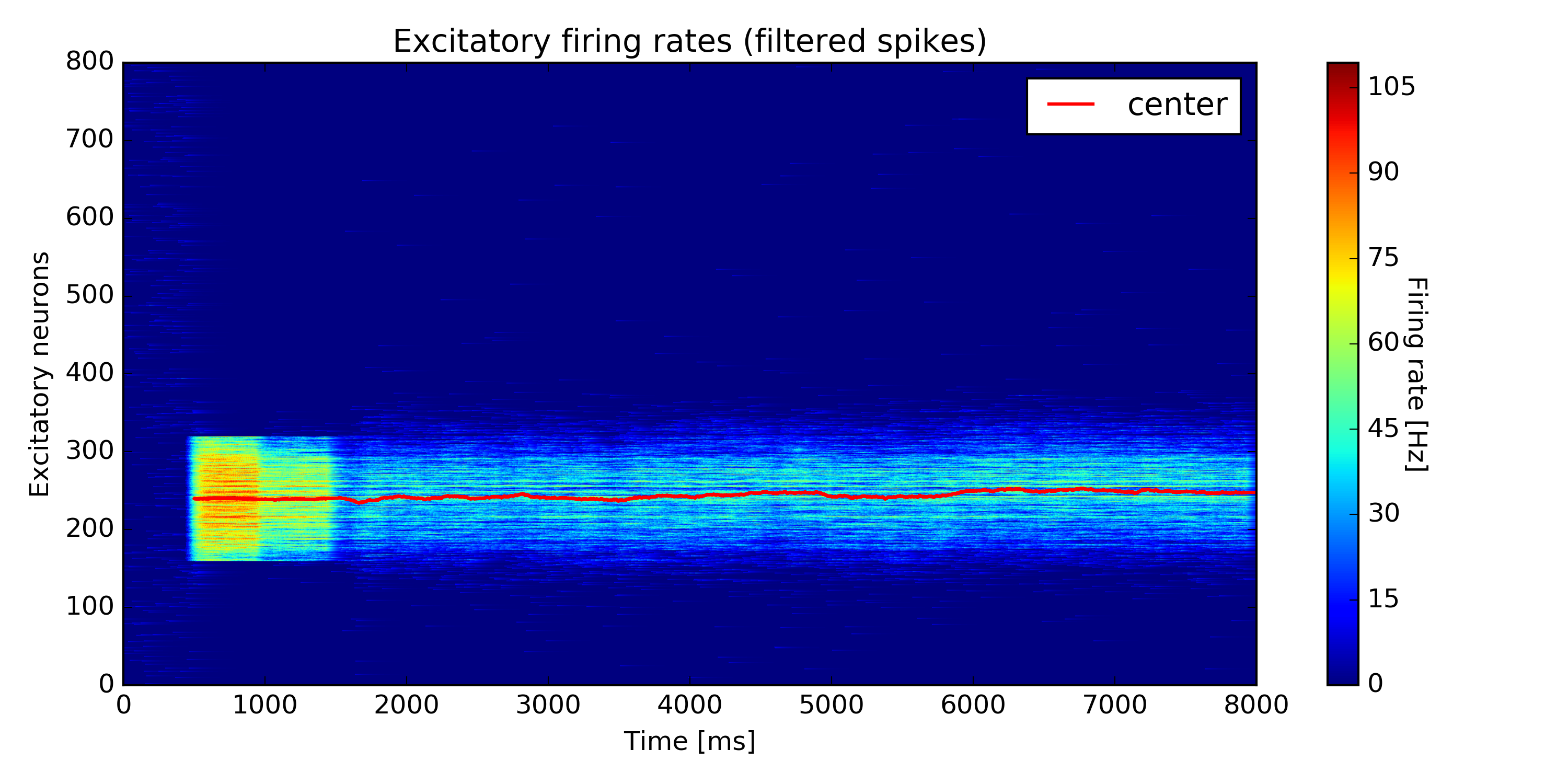
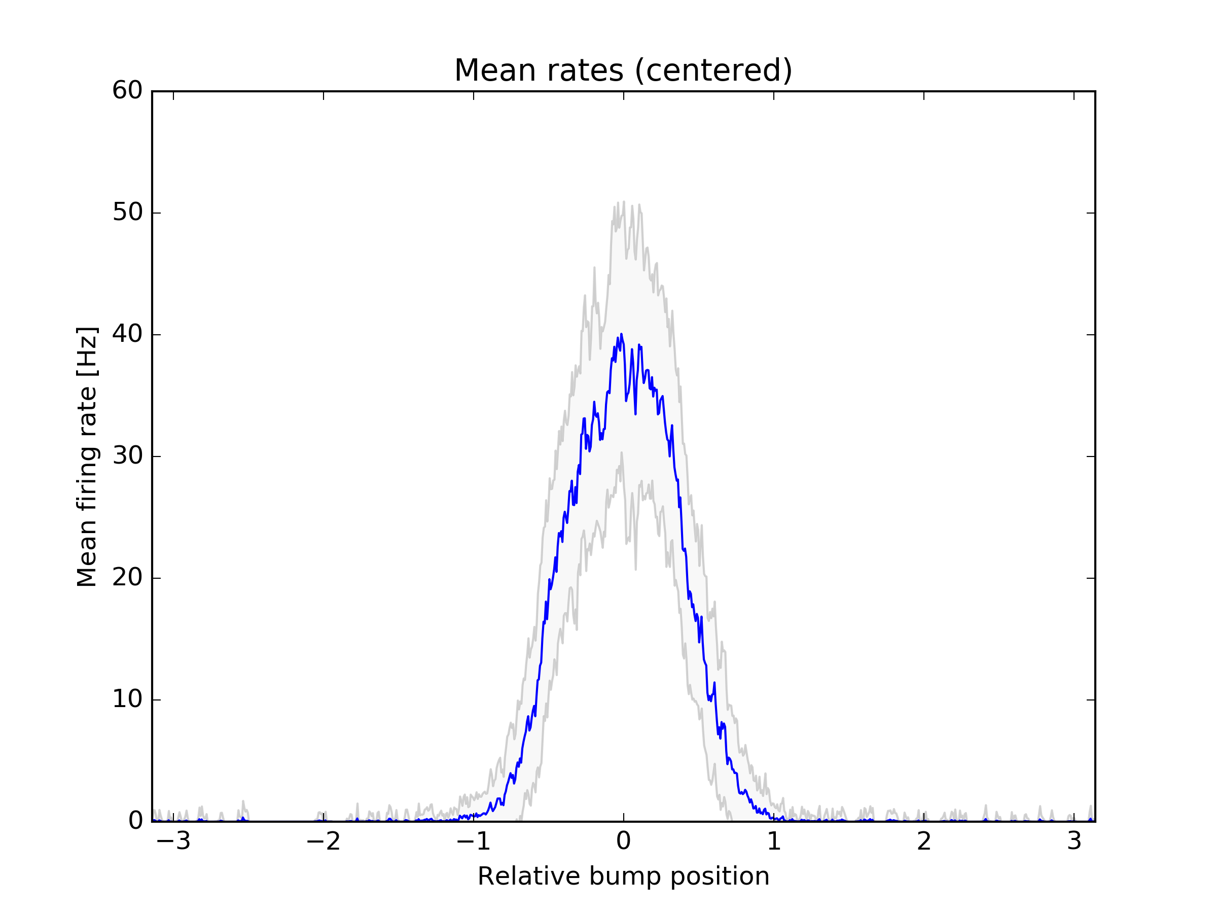
wrapper.run(handler, **sim_params)The SimBump wrapper provides the following plots after running
wrapper.plot_rates()
pl.savefig('out_rates.png')wrapper.plot_mean()
pl.savefig('out_mean.pdf')The simulation type SimDrift from simulation.sim_types implements
running several bump trajectories from equally spaced initial positions with repetitions.
To save space, this simulation type saves only bump center positions together with aggregate data, but no spike times.
This can be used to investigate the effect of different frozen noise values on the drift and diffusion of bumps, as measured by their center positions.
See scripts/run_drift.py for a demonstration of the usage of the interface. Below, we show the essential parts of this file:
import tools.db
import meanfield.error_functions as erfs
import classes.base as cb
from classes.static import MeanfieldParameters as mpr

session, net = tools.db.get_network(45)

# get meanfield handler (abstracts network parameter handling) and set connectivity parameter
handler = erfs.MeanfieldHandler(net)

# get simulation type "drift"
btype = session.query(cb.SimType).filter(cb.SimType.name == "drift").one()

# get simulation wrapper
# set to_memory = False to save simulation to hdf5 file
wrapper = btype.get_wrapper(to_memory=True, session=session)

# parameters for simulations
# this will simulate 10 initial bump positions
# with 5 repetitions each
# running until 8000 ms time each
gen_params = {
    "reps": 5,
    "tmax": 8000.,
    "initials": 10,

    # network noise parameters
    mpr.EL_NOISE: 0.,
    mpr.P_EE: 1.,  # 1mV of noise on the leak reversal potentials
    mpr.W_NOISE: 0.,

    # run parameters
    "cores": 4,  # cores to use for sim
    "tmax": 8000.,  # runtime
    "base_seed": 1,  # seed for connectivity noise
    "base_seed_run": 1,  # seed for run noise
}

# run the simulation
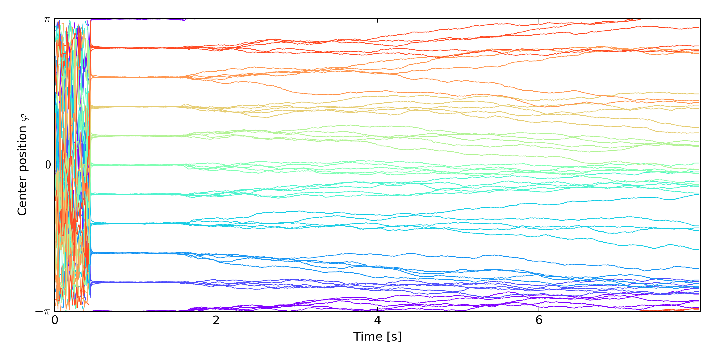
wrapper.run(handler, **gen_params)The SimDrift wrapper provides the following plots after running
Shows all bump centers of the simulated trajectories overlayed.
wrapper.plot_drift()
pl.savefig('out_drift.png')Simulations run with to_memory=False are saved in the folders data/bump
(for SimBump simulations) and data/drift (for SimDrift simulations) in the HDF5
file format. The filename is automatically generated, and is printed in the beginning of the simulation run.
The network instantiation including all parameters is saved alongside the simulation data, and can be opened as follows:
import simulation.sim_types as st
import tools.db

fn = 'data/sim/example.hdf5'  # filename
_, _, s = tools.db.db_connection()
wrapper = st.SimWrapper(data_filename=fn, session=s)  # get a general wrapper from the hdf5 file
wrapper = wrapper.sim_file.get_wrapper()  # gets the wrapper subclass instance from the file

wrapper.plot_drift()  # plot saved data
wrapper.get_gen_params()  # get parameters used for simulation

net = wrapper.sim_file.network  # get network used for simulation

