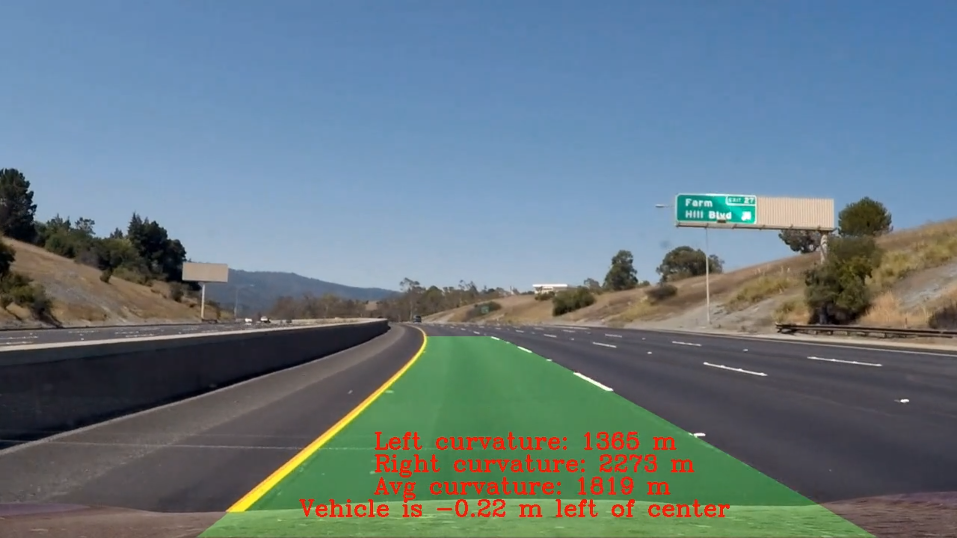
The main purpose of this project is to identify the lane boundaries in a video as in the first project of this Nanodegree. Nevertheless, this time we will face curves and difficult situations. For writing this documentation I used the writeup template which is a great starting point! Let's go!
The goals / steps of this project are the following:
- Compute the camera calibration matrix and distortion coefficients given a set of chessboard images. (this is done in the following notebook)
- Apply a distortion correction to raw images.
- Use color transforms, gradients, etc., to create a thresholded binary image.
- Apply a perspective transform to rectify binary image ("birds-eye view").
- Detect lane pixels and fit to find the lane boundary.
- Determine the curvature of the lane and vehicle position with respect to center.
- Warp the detected lane boundaries back onto the original image.
- Output visual display of the lane boundaries and numerical estimation of lane curvature and vehicle position.
The images for camera calibration are stored in the folder called camera_cal. The images in test_images are for testing your pipeline on single frames.
In order to help the reviewer examine this work I provided all the outputs from the ipython notebooks into the following folder. At the same time I will include these images into this documentation. The final output of this work is this video. I've also tested the harder challenge video, nevertheless the results are quite poor. I've also tested the challenge video. The result indicates that this sistem isn't robust when road condition changes. Nevertheless I will try to obtain a better result!
Rubric Points
Here I will consider the rubric points individually and describe how I addressed each point in my implementation.
1. Provide a Writeup / README that includes all the rubric points and how you addressed each one. You can submit your writeup as markdown or pdf. Here is a template writeup for this project you can use as a guide and a starting point.
You're reading it!
1. Briefly state how you computed the camera matrix and distortion coefficients. Provide an example of a distortion corrected calibration image.
The code for this step is contained in the following Calibrating a Camera ipython notebook.
I start by preparing "object points", which will be the (x, y, z) coordinates of the chessboard corners in the world. Here I am assuming the chessboard is fixed on the (x, y) plane at z=0, such that the object points are the same for each calibration image. Thus, objp is just a replicated array of coordinates, and objpoints will be appended with a copy of it every time I successfully detect all chessboard corners in a test image. imgpoints will be appended with the (x, y) pixel position of each of the corners in the image plane with each successful chessboard detection.
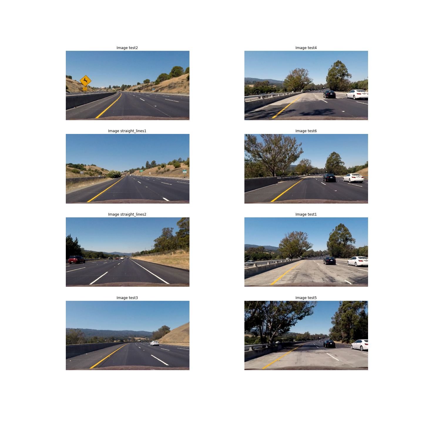
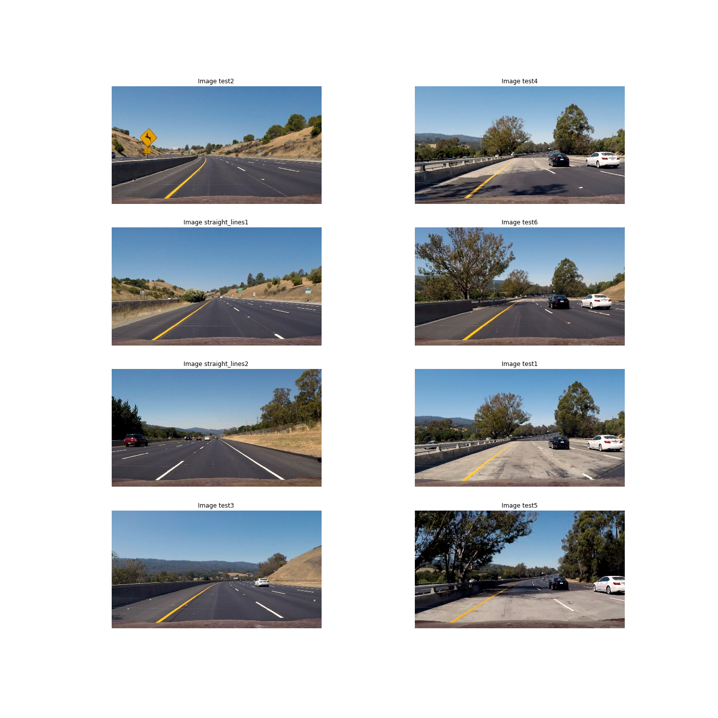
I then used the output objpoints and imgpoints to compute the camera calibration and distortion coefficients using the cv2.calibrateCamera() function. I applied this distortion correction to the test image using the cv2.undistort() function and obtained this result (all the test images undistorted):
I will also plot all the original images which I will use in order to test my implementation:
To demonstrate this step, I will describe how I apply the distortion correction (section 2) to one of the test images like this one:
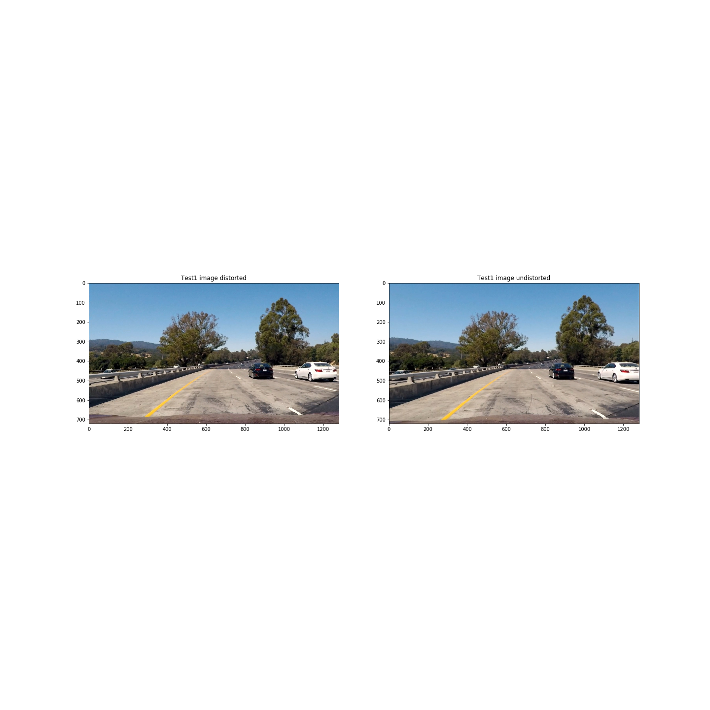
I've already included a figure with all the undistorted images, nevertheless this is a face to face distorted to undistorted where we can notice better the differences.
2. Describe how (and identify where in your code) you used color transforms, gradients or other methods to create a thresholded binary image. Provide an example of a binary image result.
All the implementation of the color transforms, gradients and other methods can be founded in the section 3.
First of all I tested different color spaces and noticed that the best choice would be by using the S channel of the HLS color space. In the following figure we can see the same figure transformed into different color spaces:
![alt_text][colorspaces]
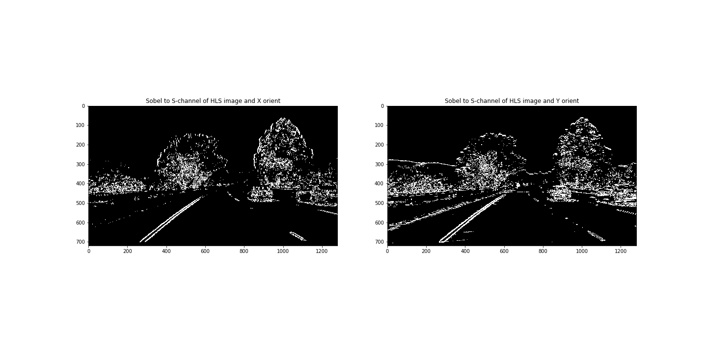
So, the first step was to tune the color thresholding process. Then, I applied sobel thresholding with both orientations as we can see the results in the following figure:
Kernel sizes where 13 for both operations and also with a min threshold of 20 and a max of 120.
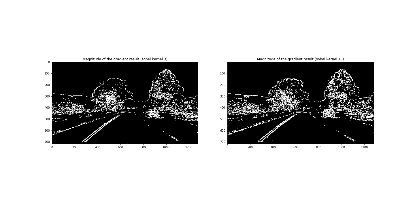
The next step was to compute the magnitude of the gradient as we can see in the following figure:
We tested two kernel sizes (3 and 15) and the threshold of (20, 100) did the trick!
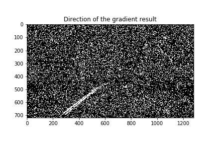
The next step was to compute the direction of the gradient:
In this case we used a high kernel size of 21 (the max is 31) and the results were quite good.
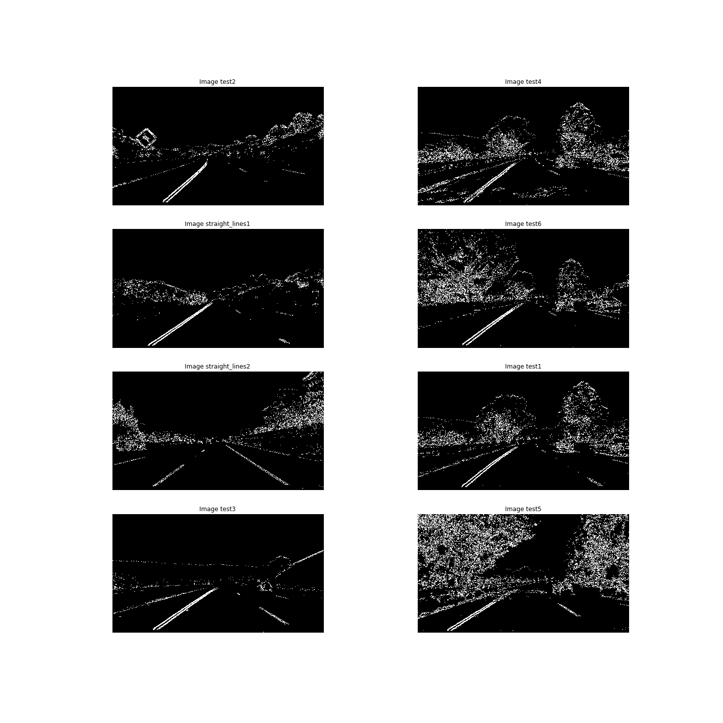
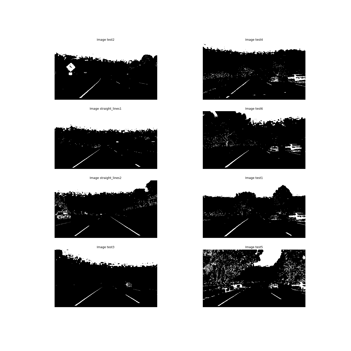
The final step of the thresholding operations was to combine all into an unique output as follows:
In the above figure we can see all the threshold operations combined for all the test images. Road lines are identified quite good, so we can proceed to the perspective transform operation.
3. Describe how (and identify where in your code) you performed a perspective transform and provide an example of a transformed image.
The code for my perspective transform includes a function called warper(), which appears in the code cell number 17 of the IPython notebook). The warper() function takes as inputs an image (img), as well as source (src) and destination (dst) points. I chose the hardcode the source and destination points in the following manner:
This source and destination points were the following:
| Source | Destination |
|---|---|
| 570, 450 | 250, 0 |
| 700, 450 | 1000, 0 |
| 1120, 720 | 1000, 720 |
| 175, 720 | 250, 720 |
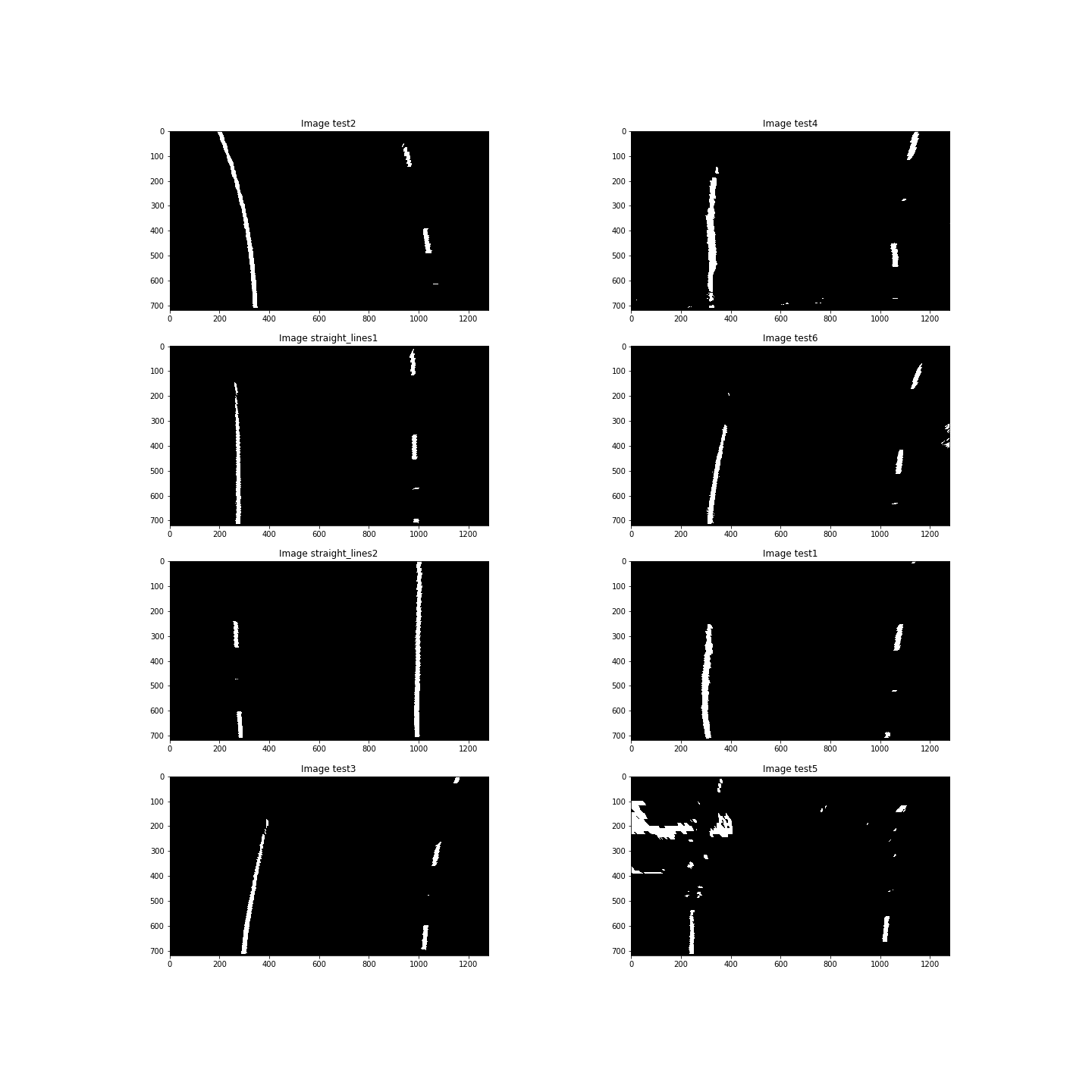
I verified that my perspective transform was working as expected by drawing the src and dst points onto a test image and its warped counterpart to verify that the lines appear parallel in the warped image. We can see the results in the follwing figure:
![alt_text][perspectivetransform]
4. Describe how (and identify where in your code) you identified lane-line pixels and fit their positions with a polynomial?
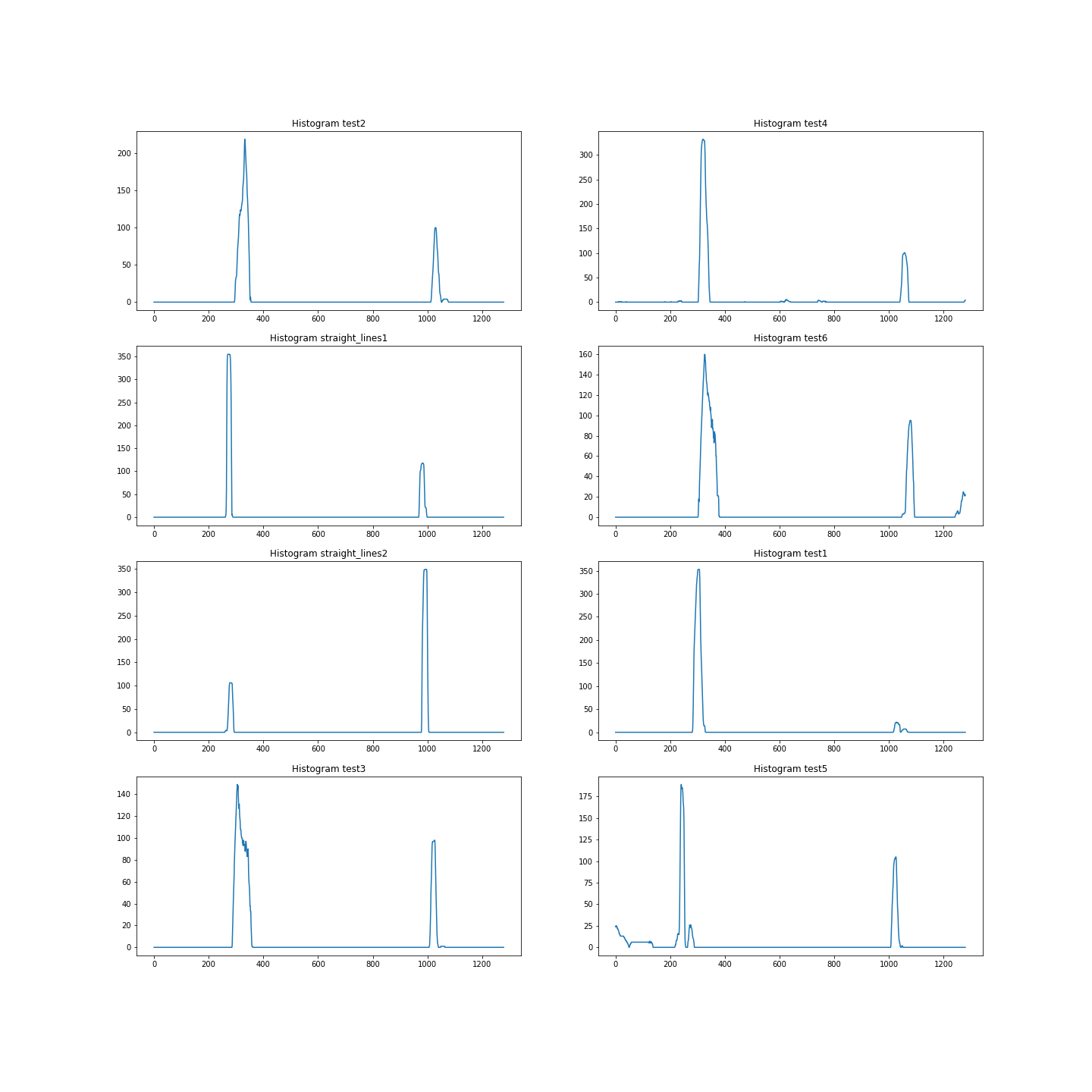
This part was implemented in the section 4. Firstly we focused on detecting the peaks in the computed histograms of the thresholded images. The histograms are the following:
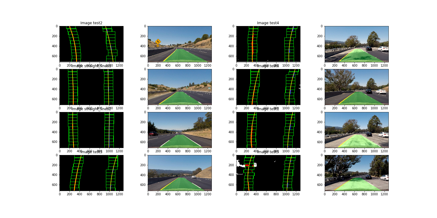
Then, we implemented the sliding window operation according to the code provided in the classroom. Basically, we firstly search the left and right peaks in the histogram corresponding to the two road lane lines. Then we identify the positions of all the nonzero pixels in the image (the input is a binary image). We next calculate the left and right lanes pixels storing the indices or pixel positions into several lists. Finally I fit my lane lines with a 2nd order polynomial kinda like this:
5. Describe how (and identify where in your code) you calculated the radius of curvature of the lane and the position of the vehicle with respect to center.
I've calculated the radius of the curvature in the section 4.4. The output was the following:
- Image test2: left curvature 1.41 km, right curvature 2.83km
- Image test4: left curvature 2.13 km, right curvature 2.32km
- Image straight_lines1: left curvature 9.56 km, right curvature 22.92km
- Image test6: left curvature 8.97 km, right curvature 5.76km
- Image straight_lines2: left curvature 10.76 km, right curvature 16.07km
- Image test1: left curvature 3.96 km, right curvature 1.63km
- Image test3: left curvature 10.73 km, right curvature 1.86km
- Image test5: left curvature 2.03 km, right curvature 1.52km
6. Provide an example image of your result plotted back down onto the road such that the lane area is identified clearly.
1. Provide a link to your final video output. Your pipeline should perform reasonably well on the entire project video (wobbly lines are ok but no catastrophic failures that would cause the car to drive off the road!).
Here's a link to my video result
1. Briefly discuss any problems / issues you faced in your implementation of this project. Where will your pipeline likely fail? What could you do to make it more robust?
The most difficult step was to choose the thresholds of the thresholding operations and also the kernel sizes. The problem is that the road lanes are not always similar and condtions changes constantly, so there is not a universal thresholding for all the situations. Also, the coose of the bounding boxes for the perspective transform was not easy. This project was challenging for me, but I've learn a lot!
Problem 1. There seems to be some confusion in the pipeline()code. The binary and warped images that are created are not distortion corrected. Distortion corrected images are made from original images but then they are not used by the following code.
True. It was a confussion into the pipeline function. My pipeline wasn't using binary undistorted images as input. I fixed this properly!
Problem 2. Some of the kernel sizes used in the above code are not valid. The only valid kernel are 1,3,5,7. https://docs.opencv.org/2.4/modules/imgproc/doc/filtering.html?highlight=sobel#sobel
Didn't know that. Need to improve my knowledge in computer vision. There is a huge lack of information :). Changed this to a valid kernel size value. Thanks!
Suggestion. I encourage you to continue trying other color spaces to isolate the yellows and whites. Try thresholding L of Luv for whites and b of Lab for yellows. By better identifying yellows and whites, the pipeline can rely less on (or avoid entirely) gradients. This is especially important and helpful for dealing with shadows and variations in the road lighting and appearance. R and V are also strong components of whites and yellows. Try to create separate thresholding strategies for whites and for yellows and then combine them.
Done. Results are much better and without using any sobel, magnitude and direction thresholding! I've implemented a function called suggested_threshold (17 code cell in the IPython notebook) using L channel of HLS, L channel of LUV and also b channel of Lab. The results are the following:
Problem 3. Nice work. Binary images are transformed to obtain a birds-eye perspective of the lane lines. The lane lines no NOT appear to be parallel. A good perspective transform is very important to obtaining good results. It is best to use an image with straight lane lines for this part of the project. If the lane lines are not transformed correctly the final polygon will have a curve when it should not.
Problem requirement 1. Try to find new source and destination points such that the lane lines appear to be parallel after transforming an image of a straight section of road.
Done, much better results when warping images! The new values are the following:
This source and destination points were the following:
| Source | Destination |
|---|---|
| 580, 460 | 250, 0 |
| 705, 460 | 1000, 0 |
| 1120, 720 | 1000, 720 |
| 175, 720 | 250, 720 |
Above image in this documentation was updated with the new one!
Problem requirement 2. The image which is used to create the warped image should be distortion corrected first (see comments above).
Done!
Suggestion. When creating the binary image it may prove helpful to create the birds-eye perspective first. The reason is that error pixels in the binary get stretched out when the birds-eye transformation is performed second.
Didn't know this! I will change it in the next commit! Thanks for the suggestion!
Some ideas to consider are :
- Are the curve estimates close in their curvature, to each other and their prior frame estimates?
- Are the lines approximately parallel?
- Are the lines approximately the correct distance apart?
- Are they approximately in the same place at their closet position to the vehicle (as the last accepted curves).
To correct this deficiency I have some suggestions:
-
Implement more/better sanity checks to reject unusable results and replace them with a result from prior frames. Some forms of averaging (of polynomial coefficients) over a few frames may be helpful. However don't over do it, because it is important to avoid reacting too slowly on curves or to changes in vehicle position within the lane. Ensure unusable frames are not averaged into the output results.
-
Continue to investigate color spaces to find a better thresholding solution. The goal is to rely more on color identification and less on gradients (which are not so useful in shadows or changing road conditions). The R and V color channels are strongly represented in yellows and whites. Try L of Luv and b of Lab also.
-
Capture images of video frames where problems are occurring and run the pipeline on those images to avoid long processing times while trying to solve a localized problem.
-
Exponential smoothing is an alternative to averaging over N frames. If you have a New frame and an Old frame, smooth by updating the New as follows: New = gamma * New + (1-gamma) * Old. 0 < gamma < 1.0
-
The pipeline uses an area around the lines fitted in prior images to search for lane pixels in a new image. Ensure the curve used to guide the search is reasonable at all times. The pipeline can be prepared to do a full blind search if usable curves cannot be found for a few frames, but don't be too quick to throw away valuable information about the expected location of likely lane line pixels. This is especially important to avoid if the thresholding is not detecting the lane lines, because all that is there will be noise.
-
Process just a particular part of the video to test troublesome areas. This example processes the frames from 39-42 seconds in
project_video:
clip_input = VideoFileClip('project_video.mp4').subclip(39,42)
clip_output = clip_input.fl_image(pipeline)
End of the project! Thanks for all the suggestions and for the exhaustive review. Was the most detailed one so far!

